Algebra and arithmetic with inductive types

As I mentioned in my previous blog post, lately I've spent a lot of time learning about category theory and type theory. One of the biggest application areas of type theory is with computer-aided proofs and proof assistants. I've found that axiomatizing the natural number system (and other more exotic number systems) in proof assistants like Agda and attempting to prove simple arithmetic identities has made me more aware of how easy it is to skip steps while doing algebraic proofs.

NOTE: a little bit of experience with Haskell or some other functional programming language would be helpful for reading this blog post.

Examples of inductive types

First, a bit of conceptual scaffolding before we get into the weeds with Agda. (If you are familiar with the basics of type theory already, feel free to skip this, or skim it as a refresher.) I won't give a full explanation of the basics of type theory here, but I'll informally introduce some concepts that are necessary to understand the motivation behind certain quirks of Agda. If you want to learn about type theory in more depth, check out the HoTT book, which I've been working through lately.

In type theory, the most basic concept is that of a type, which, intuitively speaking, is roughly analogous to a set. Types in type theory are, to some extent, meant to formalize the notion of a type as it appears in computer science and programming languages, such as the types int and char in C or the types Bool and String in Haskell. However, unlike sets, it is helpful to think of types not as completed collections of things that already exist, but rather as constraints/delimitations of things which could potentially exist, but which may or may not be "instantiated" yet. As such, types are often defined by their constructors, which are rules that allow you to produce elements or inhabitants of that type. If $a$ is an inhabitant of the type $A$, we write $a:A$, which is roughly analogous to the expression $a\in A$ in set theory. (By the way, types that are defined in terms of constructors this way are called inductive types.)

Briefly, let's consider a few examples. The familiar type of the natural numbers $\mathbb N$ can be defined by two constructors: an element $0 : \mathbb N$, and a function $\mathsf{S}:\mathbb N\to \mathbb N$, called the successor function. Starting with the element $0$, we can produce additional elements of $\mathbb N$ by repeatedly applying the constructor $\mathsf S$ to form $\mathsf{S}0, \mathsf{SS}0$, and so on. In Haskell, we could define this type as follows:

data Nat = Zero | Succ Nat

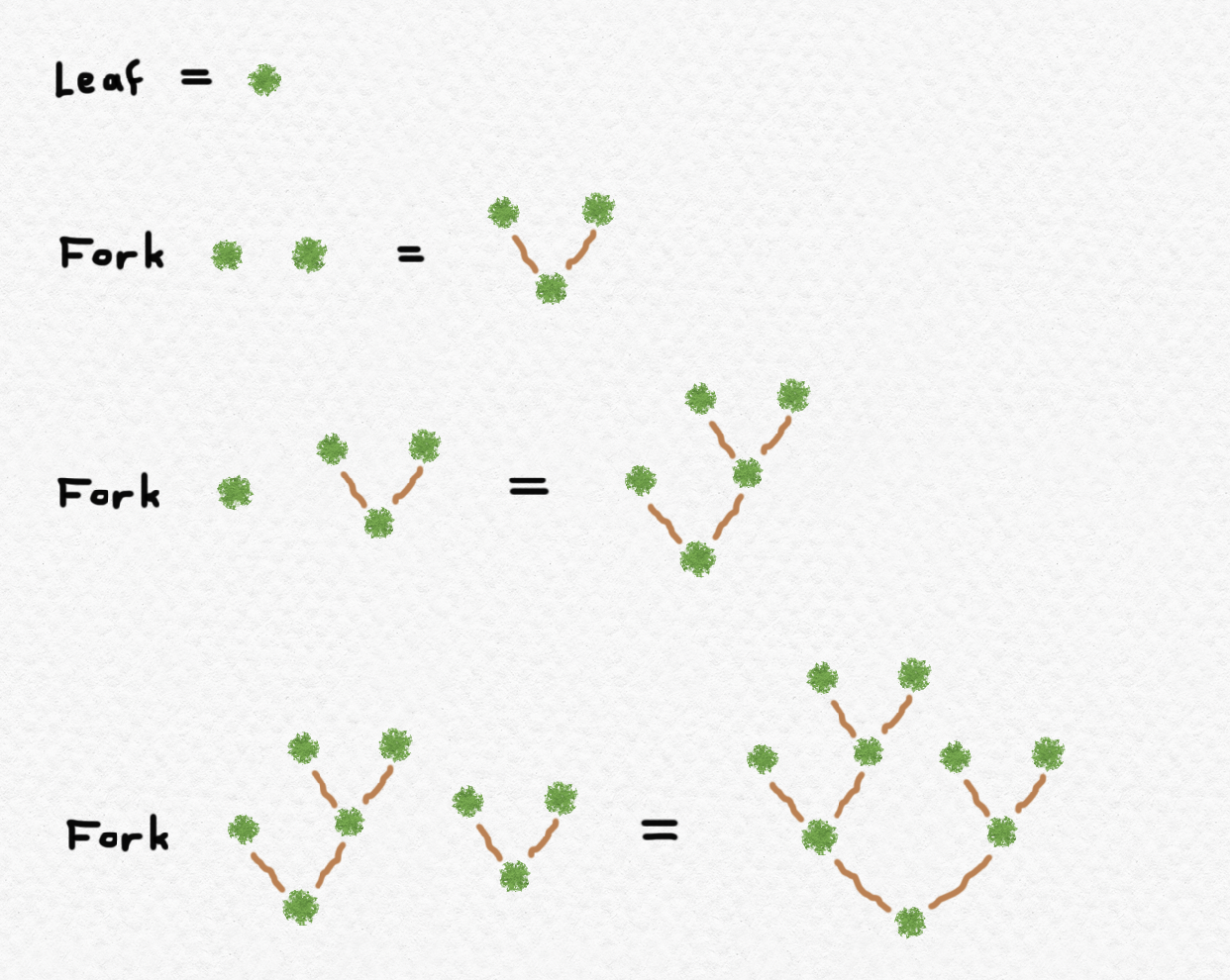
and we shall shortly see what the analogous definition in Agda looks like. For a more novel example, we could also define a type $\mathsf{BTree}$ with constructors $\text{Leaf}:\mathsf{BTree}$ and $\text{Fork}:\mathsf{BTree}\to \mathsf{BTree} \to \mathsf{BTree}$. In other words, these constructors tell us that there is an inhabitant of $\mathsf{BTree}$ called $\text{Leaf}$, and given any two inhabitants of $\mathsf{BTree}$, we can construct from them a new inhabitant of $\mathsf{BTree}$. In Haskell:

data BTree = Leaf | Fork BTree BTree

How does this abstract definition in terms of constructors have anything to do with binary trees? Here's a graphical way of interpreting it: there is, of course, a trivial binary tree consisting of nothing but a leaf, and any more complex binary tree can be thought of as a combination of two binary trees, with one to the left of the root and the other to the right of the root.

A much simpler example of an inductive type is the type denoted $\mathbf{2}$, which is called the binary type. It is inductively defined by the constructors $0:\mathbf{2}$ and $1:\mathbf{2}$. The elements $0$ and $1$ are the only inhabitants of the type $\mathbf{2}$, since there are no other constructors for this type. The binary inductive type can also double as an alias for $\mathsf{Bool}$, the type of truth-values, with $0$ representing falsity and $1$ representing truth. In Haskell, we have

data BinaryType = Zero | One

We also have a unary type denoted $\mathbf{1}$, which has only one constructor $\star:\mathbf{1}$. That is, the type $\mathbf{1}$ has a unique element. There is a nullary type $\mathbf{0}$ as well, which has no constructors at all, meaning that it is uninhabited. In other words, there is no way to construct any instance of the type $\mathbf{0}$.

Finally, there are a few different ways of defining new types from existent ones. First of all, given the types $A$ and $B$, we can form the function type $A\to B$, which is the type of functions from $A$ to $B$. To construct elements of the type $A\to B$, it suffices to define a function $f:A\to B$ using an explicit formula or a lambda expression. If $A$ is an inductive type, this can be accomplished using pattern matching, by defining the value of $f$ at every possible argument casewise depending on which constructor was used to form the argument. For instance, in Haskell, we can define a function of type $\mathsf{BTree}\to\mathsf{Int}$ like this, which counts the number of leaves of a binary tree:

numLeaves :: BTree -> Int
numLeaves Leaf = 1
numLeaves (Fork t1 t2) = (numLeaves t1) + (numLeaves t2)

We can also form the product type $A\times B$, whose analogue in set theory is the Cartesian product of $A$ and $B$, consisting of tuples $(a,b)$ where $a:A$ and $b:B$. The product type $A\times B$ can be thought of as having a constructor $(-,-):A\to B\to A\times B$: that is, given an element of type $A$ and one of type $B$, we construct an element of type $A\times B$. We also have the coproduct type $A+B$, whose set-theoretic analogue is the disjoint union. Each element of $A+B$ corresponds to either an element of $A$ or an element of $B$, so that $A+B$ can be defined by two constructors: $\text{inl}:A\to A+B$ and $\text{inr}:B\to A+B$. There are also some more techniques of type-forming, but I won't go into them here - you can read about the dependent function type and the dependent sum type in the HoTT book, if you want. (We will see examples of these in Agda later, but I won't comment on them explicitly.)

Types as propositions

The analogy between type theory and set theory breaks down when it comes to the type-theoretic treatment of logic. In set theory, logical statements about sets are sequences of characters such as $\land$ "and", $\lor$ "or", $\forall$ "for all", $\exists$ "there exists", "\in" "is an element of", etc. which follow certain syntactic rules, but which, more importantly, are external to the system of set theory itself. Syntax and semantics are separate, and making meta-theoretic statements about set theory is very difficult: it requires us to encode the logical language in set theory itself.

Type theory, on the other hand, does not use the language of first-order logic to state theorems about type theory. In type theory, types lead a double life: they can be interpreted as set-like collections of (potential) instances, or as propositions! Specifically, the type $A$ can be interpreted as a kind of "collection", or it can be interpreted as the proposition which states "there exists something of type $A$". An element $a:A$, then, also doubles as either a member of the collection $A$, or as evidence that $A$ is a true proposition, or that there does indeed exist something of type $A$. According to this interpretation, types with elements represent true propositions, whereas empty (or uninhabited) types represent false propositions. For instance, the type $\mathbf{0}$ can be thought of as the proposition "false".

Of course, we would still like to be able to represent familiar logical concepts such as "and", "or", "not", and "implies" in our new logical language. These logical operations all have equivalents in type theory. If $A$ and $B$ are types representing propositions $P$ and $Q$, the proposition $P\land Q$ "$P$ and $Q$" is represented by the type $A\times B$. Why is this an appropriate analogy? Well, to construct an element of $A\times B$, we must supply an element $a:A$ and $b:B$, which allows us to build $\text{pair}(a,b):A\times B$, and this means that both $A$ and $B$ must be inhabited by $a:A$ and $b:B$, so that $P\land Q$ is true.

What about $P\lor Q$ "$P$ or $Q$"? This proposition is represented by the coproduct type $A+B$, for to instantiate an element of $A+B$, we must use one of the constructors $\text{inl}$ or $\text{inr}$. To use $\text{inl}:A\to A+B$, we must supply an element $a:A$, and to use $\text{inr}:B\to A+B$, we must supply an element $b:B$. Thus, in order for $A+B$ to inhabited, we must have either $A$ or $B$ be inhabited, hence the parallel with the proposition $P\lor Q$.

Now, what about $P\implies Q$ "$P$ implies $Q$"? This is analogous to the function type $A\to B$. Given an inhabitant $a:A$, a function $f:A\to B$ allows us to construct an inhabitant $b=f(a):B$, meaning that if $A$ is inhabited, $B$ must also be inhabited, so that if $P$ is true, $Q$ must also be true.

Finally, what is the type-theoretic equivalent of the proposition $\neg P$ "not P"? This one is trickier and a little less intuitive. But notice that, in propositional logic, the proposition $\neg P$ is equivalent to the proposition $P\implies \text{F}$, or "$P$ implies false". And we already know that the type-theoretic equivalent of $P\implies Q$ is the function type $A\to B$, and the equivalent of "false" is the nullary type $\mathbf{0}$. Hence, $\neg P$ can be represented by the type $A\to \mathbf{0}$. In other words, the proposition $P$ is false if an element of $A$ could be used to produce an element of the nullary type $\mathbf{0}$, which is impossible by definition.

It can be a fun exercise to try and reformulate well-known tautologies from propositional logic into type-theory language, and then prove them. And how does one prove propositions in type theory? By supplying an element of the corresponding type!

For instance, consider the tautology $P\implies P$. In type theory, the corresponding proposition for a given type $A$ would be the function $A\to A$. To define a function of this type, we must come up with a way of constructing an element of type $A$, given an element of type $A$. But this is trivial: was may simply use the identity function. As a lambda function this would be $$(\lambda x . x):A\to A$$ and we can also write this in Haskell as a polymorphic function:

id :: a -> a
id x = x

As a less trivial example, consider the tautology $P\implies \neg\neg P$. The type corresponding to this proposition would be $A\to ((A\to \mathbf{0})\to \mathbf{0})$. To define a function of this type would require us to construct an element of type $\mathbf{0}$ given elements of type $A$ and $A\to \mathbf{0}$. But if we are given $a:A$ and $f:A\to\mathbf{0}$, we may evaluate $f$ at $a$ to obtain $f(a):\mathbf{0}$! Hence, we have $$(\lambda x. \lambda f. f(x)) : A\to ((A\to\mathbf{0})\to\mathbf{0})$$ which proves the proposition.

As an interesting aside, the converse of the above tautology, the law of double negation $\neg\neg P\to P$, stating that every proposition that is not-not-true is necessarily true, is not provable in type theory. The type corresponding to this proposition is $((A\to \mathbf{0})\to\mathbf{0})\to A$, and if you want to convince yourself that you can't define a function of this type, try writing a polymorphic function doubNeg :: ((a -> b) -> b) -> a in Haskell. This discrepancy between classical logic is what makes type-theoretic logic a kind of intuitionistic logic. (Another notable unprovable statement in type theory is the law of excluded middle $P\lor \neg P$.) Interestingly, however, we can eliminate a double negation from a triple negation, i.e. we can prove that $\neg\neg\neg P\to \neg P$ in type theory - this is a good exercise to try for yourself.

Reasoning about equality

There is one more piece to the puzzle that we need before we start doing algebraic proofs in Agda using type theory. We have seen how propositional logic is paralleled in type theory, but most of the statements that we wish to prove when doing arithmetic or algebra take the form $X=Y$ for some expressions $X$ and $Y$. We have not yet seen how to express statements of equality in type theory. But since all propositions are represented by types, statements of equality should as well: hence, for any type $A$ and any elements $x,y:A$, there is an equality type denoted $(x =_A y)$, which represents the proposition "$x$ and $y$ are equal as elements of $A$.

For me, understanding the equality type has been (and still is) one of the most confusing parts of basic type theory. However, for this post, there are only a few things that we need to know about it. For any type $A$ with inhabitant $a:A$, we can construct an element $\text{refl}_a:(a=_A a)$, i.e. we can assert that each element of $A$ is equal to itself, the reflexive property of equality. Additionally, for any element $p:(a =_A b)$, which we often call a path from $a$ to $b$, we can invert it to form a path $p^{-1}:(b =_A a)$, expressing the symmetric property of equality. (More generally, there is a polymorphic function $-^{-1}:(a=_A b)\to (b =_A a)$ for inverting paths.) Finally, given two paths $p:(a =_A b)$ and $q: (b =_A c)$, we can concatenate them to form a path $p\cdot q: (a =_A c)$, expressing the transitive property of equality. (There is also a polymorphic function $-\cdot -:(a =_A b)\to (b =_A c)\to (a =_A c)$.) Finally, there is a polymorphic function called $\text{ap}$ which is used to apply functions to both sides of an equality, which has the following type-signature: $$\text{ap}:(f:A\to B)\to (a =_A b)\to (f(a) =_B f(b))$$ so that the partially-applied function $\text{ap}_f$ has signature $$\text{ap}_f: (a =_A b)\to (f(a) =_B f(b))$$ allowing us to conclude that if $a=b$ as elements of $A$, and if $f:A\to B$ is a function, then $f(a)=f(b)$ as elements of $B$. These are the tools that we will need to accomplish what we want in Agda.

I said that I wouldn't get into the nuts and bolts of the equality type in this blog post, but here's a teaser: the equality types are actually inductive types as well! To define a polymorphic function over the types $(a =_A b)$ with $a,b$ ranging over the type $A$, the inductive definition of the equality type states that it suffices to define the function on all values $\text{refl}_a:(a =_A a)$, in the same way that to define a function on $\mathsf{Nat}$, it suffices to specify how it behaves on elements taking the forms $0$ and $\mathsf{S}n$. By the inductive definition of the equality type, the symmetric and transitive properties of equality are not axioms - they can be derived from the definition!

One more note before we start getting into some algebra. It might seem strangely trivial to speak of equality types $(a=_A b)$ - if $a$ and $b$ are unequal, then the type is empty, and if they are equal, the type is inhabited. What's the big deal? Well, in type theory, a great distinction is drawn between definitional equality and plain old equality. When we consider an equality type of the form $(a =_A b)$ in which $a$ and $b$ are defined by more complex expressions, they may indeed be equal, but not definitionally equal, so that some manipulation is required to show that they represent the same element of $A$. For instance, in $\mathsf{Nat}$, if $a$ is defined as $a:=\mathsf{SSSS}0$ and $b$ is defined as $b:= (\mathsf{SS}0)\times (\mathsf{SS}0)$, we will need to custom-write a function $\text{twoEq}:(\mathsf{SSSS}0 =_\mathsf{Nat} (\mathsf{SS}0)\times (\mathsf{SS}0))$ to exhibit their equality. (This is precisely the kind of manipulation that we will do in Agda.) On the other hand, if $a,b$ are literally defined in the same way, we can inhabit the equality type $(a =_A b)$ by simply using the reflexivity element $\text{refl}_a$ or $\text{refl}_b$.

Suppose that we wished to show that $\mathsf{SSSS}0=(\mathsf{SS}0)\times (\mathsf{SS}0)$, i.e. to produce an element of the identity type $(\mathsf{SSSS}0=_{\mathsf{Nat}}(\mathsf{SS}0)\times (\mathsf{SS}0))$, and that over the course of our previous manipulations, we had already procured elements of the following identity types: $$p:(\mathsf{SSSS}0=_{\mathsf{Nat}}\mathsf{SSS}0+\mathsf{S}0)$$ $$q:(\mathsf{SSS}0=_{\mathsf{Nat}}\mathsf{SS}0+\mathsf{S}0)$$ $$r:((\mathsf{SS}0)\times (\mathsf{SS}0) =_{\mathsf{Nat}} (\mathsf{SS}0+\mathsf{S}0)+\mathsf{S}0)$$ Then we can cleverly construct an element of the desired equality type $(\mathsf{SSSS}0=_{\mathsf{Nat}}(\mathsf{SS}0)\times (\mathsf{SS}0))$ using symmetricity, transitivity, and function application as follows: $$p\cdot \text{ap} _{-+\mathsf{S}0}(q)\cdot r^{-1}$$ This construction can be visualized using the following diagram:

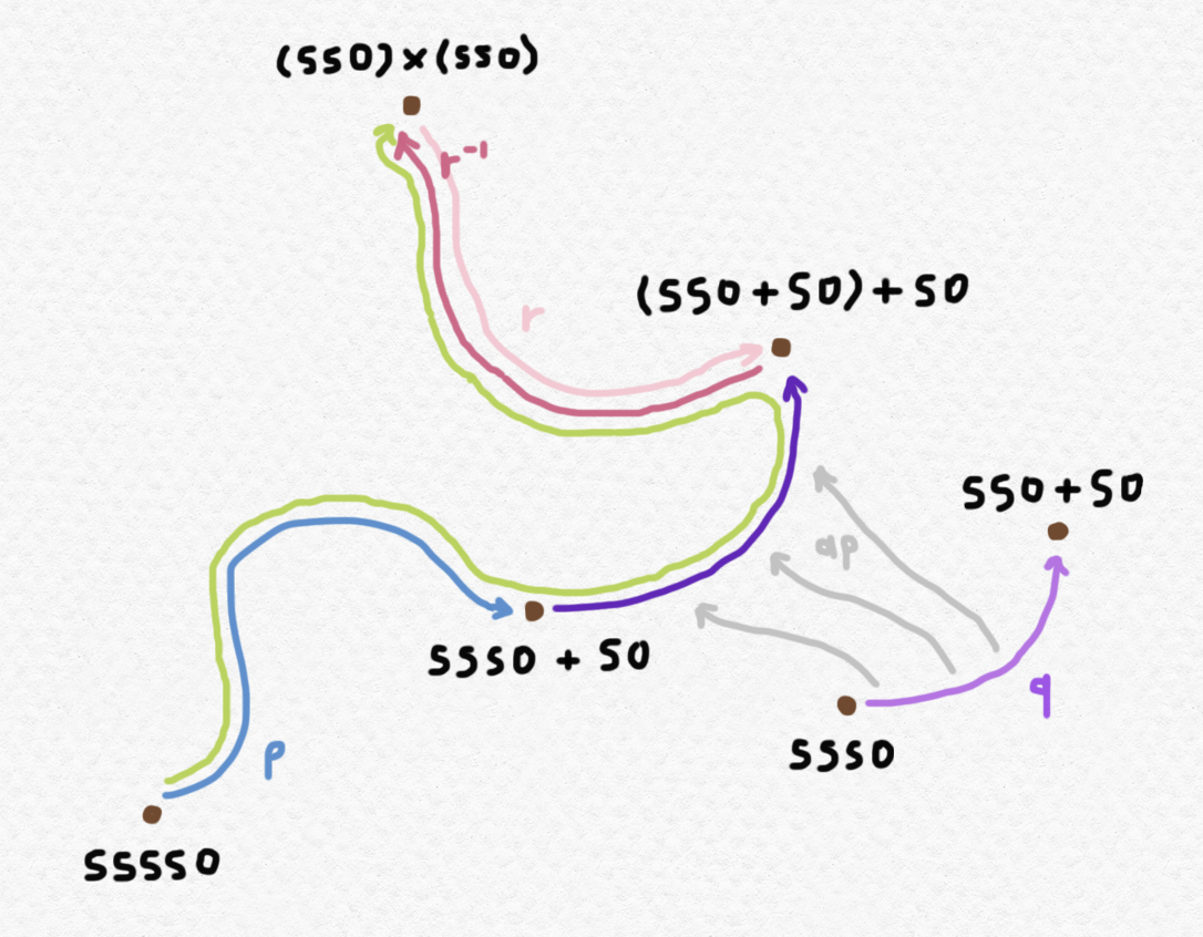
Calling elements of the equality type "paths" is more than just an unusual choice of terminology. It is often intuitively helpful to think of elements of $(a =_A b)$ as paths, even as paths of some topological space. This is the intuitive basis for the connection between topology/homotopy theory and type theory, hence the name "homotopy type theory" (often abbreviated HoTT). The analogy goes much deeper than the suggestive picture I've sketched above - but I won't go any further down this rabbit hole for now. If you'd like to learn some more about homotopy theory, you can take a look at this old blog post, in which I introduce the fundamental group of topological spaces.

Getting started with Agda

If you want to follow along with the rest of the post and play with code on your own, now's the time to install Agda. There are lots of instructions online for how to install Agda on various platforms - my laptop uses MacOS, so I used Homebrew to install Agda. You should install both agda, which will allow you to compile Agda code, and agda-mode, a plugin for the Emacs text-editor that incorporates a lot of keyboard shortcuts for typing math symbols in emacs. Most people who use Agda use this plugin and have strange unicode symbols strewn throughout their code, so if you want to build on anyone else's Agda code, this plugin is a must-have. (Unless you want to copy-paste all of the symbols into your text file - yuck!) Once you have this plugin installed, you can use this handy reference page to look up the shortcuts for various mathematical symbols. And, of course, if you're not used to using Emacs, there are plenty of resources online for familiarizing yourself with it. I personally use Vim for most things, so it's been a bit of a learning curve for me!

Now, just a few more preliminaries. Navigate to your home directory and create a directory ~/.agda. First, you should clone the Agda Standard Library into this directory. Then you'll have to create two configuration files, called defaults and libraries. In defaults, add one line containing the text standard-library. In libraries, add a line containing the absolute path to the file standard-library.agda-lib, which is contained in the agda-stdlib repository that you should have already cloned.

Wherever you please, create a directory called agda-projects or something similar, which will contain all of the Agda files that you write. Now, there are two files that you need to download into this directory, which are necessary for defining and proving some basic properties of the equality type. (You don't need to read or understand these files for the sake of this blog post, but if you're interested, they are mostly stolen from this fantastic tutorial on implementing HoTT in Agda.) The first file is Universes.agda, and the second is EqualityBase.agda.

Before you start writing your own Agda code that makes use of these two, you will need to compile them. EqualityBase is dependent on Universes, so you need to compile the latter first. Open Universes.agda in Emacs with agda-mode enables, then press Ctrl-C Ctrl-l to compile the code. (It should say "all done" at the bottom of the editor.) Then open EqualityBase.agda and do the same. For future reference, Ctrl-C Ctrl-l is the shortcut that you should use later on to compile your Agda code after making changes.

Now open a new file called whatever you want (mine is called blog_arithmetic.agda) and add two lines to the beginning like this:

module blog_arithmetic where
    open import EqualityBase public

...replacing blog_arithmetic with whatever the title of your file is (they must match, or you'll get an error). Now we're ready to start writing Agda code! For future reference, remember to indent all of your code inside of the module statement.

Natural arithmetic in Agda

It happens that the natural number type $\mathbb N$ is already defined in EqualityBase.agda, but we're going to define our own natural numbers from scratch for illustrative purposes. Here's the syntax for implementing the inductive definition of $\mathsf{Nat}$ in Agda, as we formulated it earlier:

data Nat : 𝓤₀ ̇ where
  zero : Nat 
  succ : Nat → Nat

By the way: if you're wondering about the character sequence used to type 𝓤₀ ̇, it's \MCU\_0 \^. (This tripped me up the first time I tried to write it - I couldn't figure out that there was a space between the zero and the dot.) If you're curious about what this actually is, it's essentially our universe of discourse, i.e. the higher-order type in which any other types we define will reside. The shortcut for typing the arrow → is \->.

Now let's define addition and multiplication. Because the function symbols + and ‌× are already being used in EqualityBase, we will use different symbols for the infix operations of addition and multiplication, namely ⊞ and ⊠ respectively. We can define them in much the same way as we would recursively define addition and multiplication in Haskell, using pattern matching:

_⊞_ : Nat → Nat → Nat
zero ⊞ n     = n
(succ m) ⊞ n = succ (m ⊞ n)   

_⊠_ : Nat → Nat → Nat
zero     ⊠ n = zero
(succ m) ⊠ n = (m ⊠ n) ⊞ n   

infixl 20 _⊞_
infixl 21 _⊠_

The presence of underscores on both sides of ⊞ and ⊠ in their respective definitions indicates that they are infix operations. The two lines at the end indicate that the operation ⊠ has a higher precedence than ⊞, syntactically formalizing our desired order of operations.

As an example of what proofs look like in Agda, here's a simple example, proving that $n+0=n$ for all $n:\mathsf{Nat}$. Although this may seem trivial, the equality $n+0=n$ is not definitional - we defined addition such that $0+n=n$ for all $n:\mathsf{Nat}$ (the base case of our recursive definition above), but it is not defined such that $n+0=n$. And we haven't yet proven that addition is commutative, so we can't conclude that $n+0=0+n=n$. Be careful what you take for granted!

pluszero : (n : Nat) → (n ⊞ zero) ≡ n
pluszero zero = refl zero
pluszero (succ n) = ap succ (pluszero n)

So what's going on here? By the definition of $\mathsf{Nat}$, given a natural number $n:\mathsf{Nat}$, we may assume that it is either equal to $0$ or the successor of some natural number. Thus, we may define pluszero using pattern-matching with two cases: pluszero zero and pluszero (succ n). If $n=0$, the proof is trivial, because zero ⊞ zero is definitionally equal to zero by the recursive definition of ⊞, so we may simply return refl zero. On the other hand, if the argument takes the form succ n, we can recursively call pluszero n in our definition of pluszero (succ n). Since pluszero n yields an assertion of the form (n ⊞ zero) ≡ n, we may use ap succ to apply the succ function to both sides of this equality, obtaining succ (n ⊞ zero) ≡ succ n. This is not quite what we want, since the desired type of pluszero (succ n) is ((succ n) ⊞ zero) ≡ succ n. However, notice that the types succ (n ⊞ zero) ≡ succ n and ((succ n) ⊞ zero) ≡ succ n are definitionally equal, since (succ m) ⊞ n = succ (m ⊞ n) is part of the definition of ⊞. Agda is capable of identifying these two definitionally equal types, so we may simply return ap succ (pluszero n) for the value of pluszero (succ n).

Here's a way of visualizing what is going on here, in a similar vein to the picture from before:

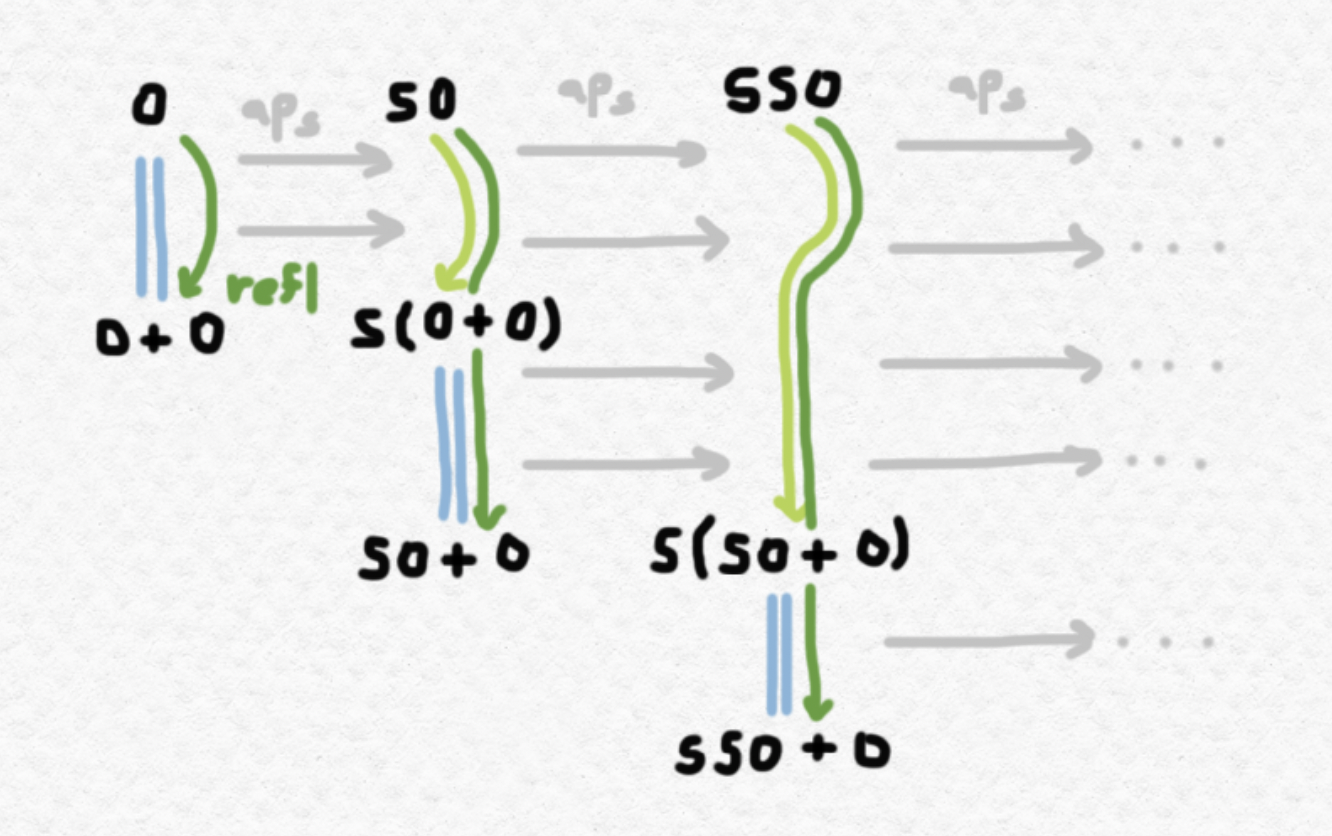
I'm using blue lines to represent definitional equalities. We start with a definitional equality between $0$ and $0+0$, then carry it over to an equality between $\mathsf{S}0$ and $\mathsf{S}(0+0)$ using $\text{ap} _\mathsf{S}$, and make use of the fact that $\mathsf{S}(0+0):= \mathsf{S}0+0$ definitionally (which Agda does automatically). Then we apply $\text{ap}_\mathsf{S}$ again and repeat the process. Note that, although we can never generate all of the equalities $n+0=n$ (since there are infinitely many natural numbers), the function pluszero allows us to generate proofs of these equalities on demand.

Now that you've seen what an example proof looks like, I'd encourage you to take a crack at proving some other simple arithmetic identity in Agda using these definitions. Try proving that addition is commutative or that multiplication distributes over addition, or perhaps something like $(n+1)(n+1)=n^2+2n+1$. You might be surprised at how often you get stuck, or how many intermediate lemmas you need! Once you've had enough, keep reading and we'll prove a couple of useful lemmas.

Let's prove three more propositions: firstly, that $\mathsf{S}n=n+1$ for all $n:\mathsf{Nat}$; secondly, that $m+(n+p)=(m+n)+p$ for all $m,n,p:\mathsf{Nat}$ (i.e. associativity of addition); and thirdly, that $\mathsf{S}(m+n)=m+\mathsf{S}n$ for all $m,n:\mathsf{Nat}$. These proofs will be much the same as the previous proof:

one : Nat
one = succ zero   

succ+1 : (n : Nat) → succ n ≡ (n ⊞ one)
succ+1 zero     = refl one 
succ+1 (succ n) = ap succ (succ+1 n)  

plus-assoc : (m n p : Nat) → (m ⊞ (n ⊞ p)) ≡ (m ⊞ n ⊞ p)
plus-assoc zero n p = refl (n ⊞ p)
plus-assoc (succ m) n p = ap succ (plus-assoc m n p)  

m-plus-Sn : (m n : Nat) → (m ⊞ succ n) ≡ succ (m ⊞ n)
m-plus-Sn zero n     = refl (succ n)
m-plus-Sn (succ m) n = ap succ (m-plus-Sn m n)

Notice that in order to formulate the former proposition, we had to first define one. However, we could have equivalently chosen to phrase succ+1 as having the type (n : Nat) → succ n ≡ (n ⊞ (succ zero)), but we're using the alias one = succ zero for the sake of conciseness.

Proving commutativity of addition - i.e. that $m+n=n+m$ for all $m,n:\mathsf{Nat}$ - will not be so straightforward. As before, we'll want to prove it inductively by making use of pattern matching on the first argument, so that our final proof will look something like

plus-comm : (m n : Nat) → (m ⊞ n) ≡ (n ⊞ m)
plus-comm zero n     = ???
plus-comm (succ m) n = ???

The base case isn't too tricky - it reduces to showing that $0+n=n+0$, and we've already shown that $n+0=n$ for all $n:\mathsf{Nat}$ with our function pluszero. This is definitionally equivalent to $n+0=0+n$, which is almost the equality we want, but backwards. This is where we'll have to use the path inversion operation that I mentioned in an earlier section:

plus-comm : (m n : Nat) → (m ⊞ n) ≡ (n ⊞ m)
plus-comm zero n     = (pluszero n) ⁻¹
plus-comm (succ m) n = ???

Now for plus-comm (succ m) n. To define this recursively, it suffices to obtain an element of type ((succ m) ⊞ n) ≡ (n ⊞ (succ m)) from plus-comm m n, an element of type (m ⊞ n) ≡ (n ⊞ m). Given that $m+n=n+m$, we can apply $\mathsf{S}$ to both sides to obtain $\mathsf{S}(m+n)=\mathsf{S}(n+m)$, which is definitionally equivalent to $\mathsf{S}m+n=\mathsf{S}(n+m)$. Additionally, we have just proven in a previous lemma that $n+\mathsf{S}m=\mathsf{S}(n+m)$. Hence, we can chain the equalities $$\mathsf{S}m+n=\mathsf{S}(n+m)$$ and $$n+\mathsf{S}m=\mathsf{S}(n+m)$$ together using transitivity to obtain the desired equality $$\mathsf{S}m+n=n+\mathsf{S}m$$ ...but how can we write this all in Agda? Well, the given element of $\mathsf{S}m+n=_{\mathsf{Nat}}\mathsf{S}(n+m)$ is ap succ (plus-comm m n), and the given element of $\mathsf{S}(n+m)=_\mathsf{Nat} n+\mathsf{S}m$ is (m-plus-Sn n m) ⁻¹, so we can concatenate these two paths to obtain (ap succ (plus-comm m n)) ∙ ((m-plus-Sn n m) ⁻¹) of type $\mathsf{S}m+n=_{\mathsf{Nat}}n+\mathsf{S}m$. Now we're ready to finish our code:

plus-comm : (m n : Nat) → (m ⊞ n) ≡ (n ⊞ m)
plus-comm zero n     = (pluszero n) ⁻¹
plus-comm (succ m) n = (ap succ (plus-comm m n)) ∙ ((m-plus-Sn n m) ⁻¹)

This compiles in Agda! Hooray!

There are plenty more things to prove about natural arithmetic in Agda, such as basic things like commutativity and associativity of multiplication and the left- and right-distributivity of multiplication over addition, or more interesting facts like the following summation identity: $$1+3+\cdots + (2n-1)=n^2$$ Another interesting puzzle is to prove more complex equalities involving associativity using only plus-assoc. For instance, as a (somewhat tedious) exercise, you might try proving that $$(((m+n)+q)+r)+s = m+(n+(q+(r+s)))$$ using only a direct definition involving plus-assoc, with no induction/pattern-matching. You might be surprised at how many steps it can take to rearrange the order of additions in expressions involving as few as just $4$ additions! (For a graphical representation of this puzzle, have a look at the associahedron.)

If you want to continue playing with natural number arithmetic by building off of the code that I've written here, but don't want to copy-paste all of it by hand, you can download blog_arithmetic.agda here.

Ordinal arithmetic in Agda

Before wrapping up, let's take a brief look at a more "exotic" number system implemented in Agda. I'd like to create a custom type for the ordinal numbers below $\omega^\omega$, with their operations of addition and multiplication. If you aren't familiar with the ordinal numbers, in short, they represent order types, which you can read about in this previous blog post. The ordinal numbers have analogues of the natural numbers $1,2,3,$ and so on, which represent finite totally-ordered sets. The ordinal $\omega$, however, represents the order type of the natural numbers. We can define an addition operation on order types which consists of "concatenating" two order types together, and a multiplication operation, which consists of substituting the elements of one order with copies of another. (You can read about both of these operations in the blog post linked above.)

Unfortunately, there's no hope for implementing a data type that allows us to construct all ordinals, since there are uncountable ordinals (and even the countable ones can get pretty crazy), but I'll show how to implement the ordinals below $\omega^\omega$: that is, the ordinals that can be represented as polynomials in $\omega$, such as $\omega^4\cdot 3 + \omega\cdot 5 + 1$. Just as every natural number can be uniquely represented by a sequence of successor operations applied to $0$, every ordinal of this form can be represented uniquely by a sequence of successor operations and multiplications by $\omega$ applied to $1$. For instance, $$\omega^4\cdot 3 + \omega\cdot 5 + 1=\mathsf{S}(\omega\times \mathsf{SSSSS}(\omega\times\omega\times\omega\times 1))$$ Hence, we can represent these ordinals using an inductive type called ωpoly with one starting element one : ωpoly and two unary constructing functions _+1 : ωpoly → ωpoly and ω×_ : ωpoly → ωpoly. My definition for ωpoly is as follows:

data ωpoly : 𝓤₀ ̇ where
    one : ωpoly
    _+1 : ωpoly → ωpoly
    ω×_ : ωpoly → ωpoly

Defining addition and multiplication for ordinals of this form is a little trickier than with the natural numbers, since there are more cases to consider: when pattern matching, an arbitrary element of ωpoly could take any one of the three forms one, m +1, and ω× m. Here's the definition that I came up with for addition:

_⊞_ : ωpoly → ωpoly → ωpoly
m      ⊞ one    = m +1
m      ⊞ (n +1) = (m ⊞ n) +1
one    ⊞ (ω× n) = ω× n
(m +1) ⊞ (ω× n) = m ⊞ (ω× n)
(ω× m) ⊞ (ω× n) = ω× (m ⊞ n)

The third and fourth cases are motivated by the fact that the ordinal $\omega$ absorbs addition with $1$ on the left. That is, concatenating a single element at the beginning of the order type of $\mathbb N$ leaves the order type the same. The fifth case states intuitively that $m$ copies of $\omega$ followed by $n$ copies of $\omega$ is the same as $(m+n)$ copies of $\omega$.

Here's my definition of multiplication for ordinals:

_⊠_ : ωpoly → ωpoly → ωpoly
(ω× m) ⊠ n      = ω× (m ⊠ n)
m      ⊠ one    = m
m      ⊠ (n +1) = (m ⊠ n) ⊞ m
one    ⊠ (ω× n) = ω× n
(m +1) ⊠ (ω× n) = m ⊠ (ω× n)

I've managed to prove that under these definitions, ordinal addition is associative, and I'm currently working on a proof that multiplication is left-distributive over addition. An interesting fact, however, is that it is not right-distributive over addition. Nor are addition and multiplication commutative! So ordinal arithmetic is quite different from arithmetic with the natural numbers. Nevertheless, there are plenty of interesting algebraic identities to be proven, such as the following (courtesy of Sierpinski): $$(\omega^3+\omega)^5 = (\omega^5+\omega^3)^3$$ and the following (which comes from my own generalization of Sierpinski's exercise): $$(\omega^{201}+\omega^{102})^{100}=(\omega^{100}+\omega)^{201}$$ As of right now, my goal is to build up the theory of ordinal arithmetic on $\omega^\omega$ in Agda to a sufficient extent that I'm able to prove Sierpinski's identity $(\omega^3+\omega)^5 = (\omega^5+\omega^3)^3$. Perhaps this will be the subject of a future post!

Summary

Initially, I had wanted to write a short post exploring several different systems of arithmetic in Agda. However, once I started writing, it occurred to me that there are a lot of formal and conceptual prerequisites for motivating and understanding the style of Agda, so it ended up turning into an intuitive introduction to type theory and getting set up with Agda instead. Now that I've written this up, maybe I'll be able to get deeper into the weeds in future posts.

As an aside, this summer I'll be a counselor and mentor at PROMYS, a summer program for highschoolers at Boston University that introduces formal/rigorous proofs and several topics in number theory and abstract algebra. I actually attended this program as a highschooler, and benefitted greatly from all of the new ideas that I was exposed to there. Part of what the program encourages students to do is prove what they know about arithmetic and $\mathbb N$ "from the ground up", starting with a collection of axioms and taking nothing else for granted, no matter how "obvious" it may seem. As I work with my high-school mentees at PROMYS, it might be fun to try and follow along by proving some of the same results about number theory and abstract algebra in Agda! This would certainly be in keeping with the idea of being explicit about our assumptions and proving everything else from the ground up.