Lately I've been brushing up on my statistics (which is only prudent given all of the buzz about ML in the software dev world right now) and I've gone down a bit of a rabbit-hole studying parameter estimation problems. Lehmann's books Theory of Point Estimation and Testing Statistical Hypotheses present parameter estimation problems in a general framework that I've found pretty insightful. Actually, as a side project I've put together a little website with a collection of parameter estimation challenges that you can solve in the browser by writing a WebR function. Check it out!
These parameter estimation problems involve making estimates of unknown quantities given only imperfect information in the form of randomly distributed data. Penalties for incorrect answers are calculated in terms of a given "loss function". An interesting subclass of these problems are the minimax problems, where you are tasked with minimizing the expected loss in the worst case, that is, minimizing the maximum possible expected loss across all possible values of the unknown quantity.
Lehmann comments that minimax problems are often very tricky to solve compared to other forms of parameter estimation problems. Of course, I had to see this for myself to believe it, so I wrote down one of the simplest minimax problems I could think of and tried to solve it.
And boy, was he right. I've been toying with this problem on and off for the past several weeks, and it's been infuriating, particularly because the problem's statement is so simple on its face. But I finally finished solving it analytically just a few days ago, and the solution is far more complicated than it has any right to be.
Anyways, here's the problem:
There is an unknown parameter $\vartheta \in [0,1]$, and you need to make a guess $\vartheta^\ast$ at the value of this parameter. You are penalized based on how far off your guess is from the true value - if the true value is $\vartheta$ and your guess is $\vartheta^\ast$, then the penalty is $L(\vartheta,\vartheta^\ast) = (\vartheta - \vartheta^\ast)^2$, that is, the squared error. The only information you are given to inform your estimate is the value of a random variable $\omega\sim \mathcal U(0,\vartheta)$, that is, the value of a uniformly distributed random value in $[0,\vartheta]$.
How can you choose your estimate in order to minimize the maximum possible expected penalty? That is, what strategy will guarantee the expected penalty to be as small as possible, regardless of the true value of $\vartheta\in [0,1]$? And what is this smallest possible expected penalty?
The "strategies" for solving this problem can be represented as "decision functions" $\delta: [0,1]\to [0,1]$ such that $\delta(\omega) = \vartheta^\ast$ gives an estimate for the parameter $\vartheta$ in terms of the random observation $\omega\sim \mathcal U(0,\vartheta)$. You can take a crack at this problem yourself on my website by writing a decision function in R, if you want.
This post will describe the winding path that I followed to the ultimate grotesque solution of this minimax problem. Enjoy! 🤡
In Lehmann's Theory of Point Estimation, he mentions a very useful fact about minimax problems: if you can find a prior distribution $\Lambda$ and a Bayes solution $\delta_\Lambda$ for that prior that makes the risk function a constant function, then $\delta_\Lambda$ is automatically a minimax solution for the problem. (The risk function $R(\delta, \vartheta)$ is defined as the expected loss when a specific decision function $\delta$ is used, and the true parameter value is $\vartheta$.) He shows how to use this fact to deduce the minimax estimate for an unknown parameter $p$ given a binomially distributed random variable $X\sim\text{Binom}(n,p)$. (He does this by letting $\Lambda$ be a certain beta distribution, but as for where this idea came from in the first place, he kind of pulls it out of a hat.)
So naturally, my first step was to look for a decision function $\delta$ making the risk function $R$ constant. Then I could try to find a prior distribution for which that decision function was Bayes optimal, and my work would be done. For the risk to be constant as a function of the parameter $\vartheta$, the following expression would have to be constant as a function of $\vartheta$:
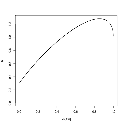
It took me a few weeks of on-and-off work on this problem to realize that $\delta$ can be solved for analytically. But in the meantime, I found an approximate solution for $\delta$ by discretizing the interval $[0,1]$ into a bunch of evenly spaced points and reformulating the problem as a system of linear equations that could be solved algorithmically. In fact, there are infinitely many solutions $\delta$, as for any particular solution $\delta$, another solution can be obtained from the function $x\mapsto \alpha \delta(x/\alpha)$ for any $\alpha > 0$, dilating the solution about the origin. This yields a function looking something like this:
This poses an unfortunate problem: there is no way to dilate/contract this function in such a way that it is defined on all of $[0,1]$ and is also $\leq 1$ everywhere on $[0,1]$. This means that $\delta$ cannot be the Bayes solution for any prior $\Lambda$, because it can never be optimal to guess a value of $\vartheta$ that is greater than $1$ (since $\vartheta$ only takes values in the interval $[0,1]$). This dashes any hopes of proving minimaxity via the aforementioned theorem on constant risk functions.
Of course, we could always try modifying this decision function so that it never returns an "unreasonable" estimate $\vartheta^\ast > 1$. For instance, we might consider a decision function $x\mapsto \min(1, \delta(x))$ where $\delta$ is the function depicted above that makes the risk function $R$ a constant function. But of course, this truncated version does not make the $R$ a constant function. If we use $x\mapsto \min(1, \delta(x))$ as our decision function, then the new risk function looks like this:
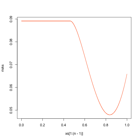
The maximum risk here is approximately $\approx 0.0891$, which is not too bad! But this risk function is non-constant, so there is no guarantee of minimaxity. And as we shall see in a moment, it is not, in fact, optimal.
After (erroneously) deciding that it was unlikely I would ever analytically find a minimax solution to this problem, I started looking for approximate numerical solutions. Initially, I had used numerical methods to approximate a decision function $\delta$ making the risk function constant. But a more direct approach would be to numerically calculate a decision function $\delta$ minimizing the maximum value of the risk function $R(\vartheta)$ by using a numerical minimization method.
My numerical approach to this problem was as follows:
There is a bit of a problem with this approach, though. Although the risk $r(\delta)$ is a differentiable function with respect to the different components of the $\delta$ vector, the supremum norm $\lVert\cdot\rVert_\infty$ is not a differentiable function of its vector argument, so gradient descent cannot really be applied (in its usual form) to the objective function $\delta\mapsto \lVert r(\delta) \rVert_\infty$.
Instead, I applied a modified form of gradient descent in which at each step, only the gradient of the largest component of $r(\delta)$ is calculated and used to adjust the input vector $\delta$. This way, each step of the gradient descent algorithm focuses on decreasing the largest component of the output risk vector $R = r(\delta)$, which is necessary to decrease the maximum component of the vector $R$.
This was just my heuristic approach to the problem, and it yielded a helpful insight, as we will see in a moment. But there was nothing rigorous about this idea. I've found no reference to this modified sup-norm version of gradient descent anywhere online, so I have no idea if there are any theoretical guarantees of its convergence. Also, the usual gradient descent algorithm uses the gradients at previous steps to dynamically adjust the step size, but because my modified algorithm is constantly switching between different components of $R$ to minimize, this kind of intelligent step size calculation wasn't possible. Instead, I just picked a "small enough" static step size to see what the method would turn up.
Here's an animation of my modified gradient descent algorithm being applied to an initial decision function guess of $\delta(x) = x$:
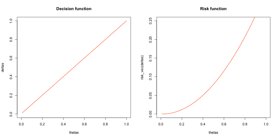
We can see the input decision function $\delta$ and the output risk function $R$ seemingly converge to functions shaped similarly to what we saw in my original failed attempt. To me, this suggested that my initial approach might not have actually been too far off. However, the maximum risk of this numerical solution was significantly lower at $\approx 0.0747$, as compared to a maximum risk of $\approx 0.0891$ in the original attempt.
The risk functions for the original attempt and this newer attempt look similar, in that they consist of a plateau stretching until about $x\approx 0.5$ followed by a parabolic-looking dip downwards. However, a notable difference between them is the fact that in the older solution, the end of the dip at $x=1$ falls short of the height of the original plateau, while in the newer solution, the end of the dip at $x=1$ seems to match the height of the original plateau. This qualitative observation led to the conjectured exact solution described in the next section (later proven to be correct).
Previously, I mentioned the idea of trying to "salvage" a non-Bayes (and non-admissible) decision function $\delta$ making the risk function $R$ a constant function by capping its values at $1$. Then, when I used a modified version of gradient descent to search for a minimax solution, I noticed that the apparent numerical solution (and its risk function) looked an awful lot like the solution and non-constant risk function that I had salvaged from my original attempt, except that the height of the plateau in the risk function starting at $R(0)$ appeared to align with the final value $R(1)$ of the risk function.
This led to my next method of attack: trying to find a decision function which both makes $R$ constant, and also makes $R(0) = R(1)$ when it is "capped" at a maximum value of $1$. In what follows, I will let $f$ denote a non-admissible decision function that makes $R$ constant, and let $\delta$ denote the decision function that results from capping it off at a maximum value of $1$.
Around this time is when I figured out how to analytically solve for functions $f$ reducing the risk function $R$ to a constant, by solving a certain differential equation. And the answer is weird.
We're looking for functions $f$ satisfying the following integral identity, for some constant $C$: Note that this is the same as saying Using the Leibniz integral rule we can turn this into a differential equation for the function $f$: we obtain From this point, the calculations are a big nicer if we make a substitution, considering the function $g$ defined as $g(\vartheta) = f(\vartheta) - \vartheta$ in place of the function $f$. With this substitution, the above becomes Differentiating once more with respect to $\vartheta$ yields: or, after simplifying,
The solution to this differential equation is quite messy and involves defining $g$ implicitly. (To be completely honest, I found the solution at first using Wolfram, but came up with the following slick derivation after the fact.) To solve it, we'll first define a complex-valued function $z:(0,1)\to \mathbb C$ as $z(\vartheta) = \zeta_3\vartheta + g(\vartheta)$, where $\zeta_3$ is the complex cube root of unity in the upper half-plane. Then note that by the differential equation for $g$, we have which means that the following quantity has to be purely real, since $g$ is a real-valued function: But note this is simply the derivative of $\zeta_6^{-1}\log(z)$. Thus, since the derivative of $\zeta_6^{-1}\log(z)$ with respect to $\vartheta$ is a purely real quantity, the derivative of its imaginary part with respect to $\vartheta$ vanishes, and we have that it must have constant imaginary part: By decomposing $z$ into its real and imaginary parts in terms of $g$ and $\vartheta$ and computing the imaginary part of $\zeta_6^{-1}\log z$ in terms of these quantities (and simplifying a bit, absorbing some numbers into the arbitrary constant $C$), we obtain the following gross-looking definition for $g(x)$ as an implicit function of $x$:
Nasty! But if you open up a graphing calculator and plot the curve defined by this equation:
you will miraculously find a shape that looks just like the graph we saw earlier.
As discussed before, the empirical results of my (sus) gradient descent had led me to believe that the true minimax solution is a truncated version of the decision function $f$ (for some value of the constant $C$) defined as follows, where $x_\ast$ is the smallest real value $x$ for which $f(x) = 1$, i.e. the point at which $f$ turns into a decision function that no longer makes sense: and further, that $\delta$ it is such that its risk function $R$ satisfies $R(0) = R(1)$. It turns out that we can actually calculate the exact value of the constant $C$ (and hence the implicitly defined function $f$) for which this condition on the risk function is satisfied. This condition is equivalent to or, since $\delta = 1$ for all $x\geq x_\ast$, the condition is Using the properties of $f$ and the differential equation for $g$, the RHS can actually be reduced to a pretty simple form in terms of $x_\ast$. I'll leave the details as an exercise, but it can be shown that the RHS can be reduced to the simple expression $f_0^2 - (1-x_\ast)(2x_\ast^2 - 3x_\ast + 1)$, from which it follows that the above equation implies The only solution to this equation other than $x_\ast = 1$ (which is not possible) is $x_\ast = 1/2$ - a remarkably simple answer to a very complicated question! This means that if the condition $R(0)=R(1)$ holds then we must have $x_\ast = 1/2$, and consequently $f(1/2) = 1$, or $g(1/2) = 1/2$. Setting $(x,g) = (1/2,1/2)$ in the implicit equation defining $g(x)$ gives the following value of the constant $C$: which yields the following minimax loss value: which agrees numerically with the minimax loss value that I found empirically.
After a few weeks of banging my head against the wall, I wasn't expecting to find an exact value for the minimax expected loss at all. And if I had, I certainly wouldn't have expected that kooky number!
At this point, I had a numerical minimax solution, and I had an analytical description of a function agreeing with it numerically which I conjectured to be minimax. But still no proof of its minimaxity.
But finally I realized that another result from Lehmann on minimax solutions could still be applied, since it had slightly weaker hypotheses. In the weaker theorem, the risk function $R$ is not required to be constant. It is just required to be constant on a set of unit measure with respect to the prior distribution for which $\delta$ is Bayes. That is, $\delta=\delta_\Lambda$ needs to be a Bayes solution for some prior distribution $\Lambda$, and the risk function $R$ only needs to be constant on some subset $A\subset [0,1]$, so long as that subset has probability $\Lambda(A) = 1$.
The solution $\delta$ that we've constructed above has a risk function $R(\vartheta)$ that is not constant. However, it is constant on the set $[0,1/2]\cup {1}$. This result means that if we can find a prior distribution $\Lambda$, supported on the set $[0,1/2]\cup {1}$, for which $\delta=\delta_\Lambda$ is the Bayes solution, then $\delta$ is in fact minimax. And this time, there are no glaring red flags about $\delta$ that preclude it from being minimax.
The most general prior distribution $\Lambda$ supported on $[0,1/2]\cup {1}$ takes the form $\Lambda(X) = p [[ 1\in X ]] + (1-p)\Lambda_0(X)$ where $p\in [0,1]$ and $\Lambda_0$ is a narrower distribution on the set $[0,1/2]$. That is, a random variable on the set $[0,1/2]\cup {1}$ must take the value $1$ with some probability $p\in [0,1]$, and must follow some other distribution $\Lambda_0$ when its value falls in the interval $[0,1/2]$.
We shall try to choose $p$ and $\Lambda_0$ in order to make our $\delta$ the Bayes solution for $\Lambda$. When the squared error loss function is used, the Bayes solution is just the expected value of the posterior distribution, meaning that
when $x\in [0,1/2]$. When $x > 1/2$, of course we have that $\delta_\Lambda(x) = 1$, since an observation of $1$ means that the value of $\vartheta$ must be $=1$ when it is known to belong to $[0,1/2]\cup {1}$. So we want to choose a value of $p$ and a density function $\Lambda_0$ such that the above equals $f(x)$ for all $x\in [0,1/2]$.
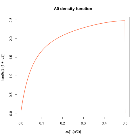
With a bit of algebra, this can be turned into a nice differential equation for $\Lambda_0$. I found the following solution: where I'm not sure if this integral representation for $h$ in terms of $f$ can be simplified any further using the differential equation for $f$ - perhaps it can. But the above is sufficient to show existence of a Bayes prior $\Lambda$ for which $\delta = \delta_\Lambda$. One can check that the above does in fact define a valid density function for $\Lambda_0$ - namely, $\Lambda_0$ is positive on $[0,1/2]$ and it has unit integral over that interval - and that it satisfies the requisite integral equation to ensure $\mathbb E_\Lambda[\vartheta|x] = f(x)$ for $x\in [0,1/2]$. Just to get an idea of what this distribution looks like, here's the density function $\Lambda_0$ on $[0,1/2]$:
and the value of $p$ is approximately $\approx 0.713$.
This gives us a final definitive answer: the function $\delta$ is indeed a minimax solution of our problem. Whew!
That wraps up my extended treatment of this problem. I really was not expecting to find exact expressions for the minimax solution and minimax expected loss, and I'm blown away by how strange-looking they are. I also wasn't expecting to encounter such tricky differential equations.
Overall, a damn cool problem!