Supply and Demand are the two most important concepts in microeconomics, and in this post I will define both, explain how they work and interact with each other, and explore some interesting theoretical scenarios related to Supply and Demand.
Our discussion of Supply and Demand takes place in a market for some generic good (steel, breakfast cereal, medicine, etc), so before we start to explore Supply and Demand we must identify a few types of goods and their relationships. A normal good is a good that consumers consume in greater quantity as their income increases. Most goods are normal, and the exceptions are inferior goods, which consumers purchase in lower quantity as their incomes rise. Examples of inferior goods include used clothing, since people who can afford to buy new clothing typically prefer to do so.
Two goods are called complements or complementary goods if their consumption increases or decreases together, or if they usually are consumed together. Cereal and milk, hammers and nails, and hamburgers and buns are all pairs of complementary goods. Substitute goods, on the other hand, can stand in for each other and are somewhat interchangeable in the eyes of consumers. Examples of pairs of substitute goods might include ketchup and mustard, coffee and tea, or pencils and pens. If, for some reason, one good becomes unavailable to consumers (due to high prices, shortage, or something else), they will consume a greater amount of its substitute good if any exists.
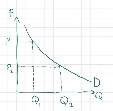
Now we are ready to begin our discussion of Supply and Demand. Let’s start with demand, which is defined as the relationship between the price of a good and the quantity of the good that consumers will collectively purchase. In other words, demand is a function mapping possible good prices to quantities purchased by consumers at each of the respective prices. Demand is represented graphically by a demand curve with price $P$ on the $y$ axis and quantity $Q$ on the $x$ axis:
The above graph is an example of a demand curve, with two points $(Q_1, P_1)$ and $(Q_2, P_2)$ shown explicitly. A literal interpretation of this graph would be that if the market price of good X is $P_1$, then the quantity demanded by consumers will be $Q_1$, while a market price of $P_2$ corresponds instead to a demanded quantity of $Q_2$. Note that the negative slope of the curve indicates that the greater a good’s market price is, the smaller the quantity demanded will be, as we would expect. This fact is called the Law of Demand (there are exceptions to this rule, called Giffen Goods, but I won’t talk about them in this post). If the price of peanut butter miraculously drops, people will rush to the store to take advantage of the deal. If the price of peanut butter rises, people will find something else to spread on their sandwiches.
Notice that according to the above definition, $Q$ is a function of $P$, yet $Q$ is assigned to the $x$-axis, where the independent variable usually resides. This is simply a convention used by economists, and there is no real justification of this convention to my knowledge.
Now for an explanation of supply, which is the relationship between the market price for a particular good and the quantity of that good that producers are willing to (can afford) to sell at that price. Typically, if the market price for a good is higher, there is a greater opportunity for firms to produce the good and sell it at a profit, so the quantity supplied will be greater. Conversely, if the market price for a good is low, fewer firms can produce the good at a low enough cost to sell it at such a low price for a profit, so the quantity supplied will be smaller. If you’re running a pizza parlor and it costs you $10$ dollars to make one pizza, you won’t be able to afford to sell pizzas for anything less than $ $10$. So when Little Caesar’s takes the pizza market by storm with a miraculous technology that converts cardboard boxes into pizzas at a cost of $50$ cents per pizza, people will flock to Little Caesar’s and the market price of pizza will plummet, putting you and your quaint pizza parlor out of business for lack of customers willing to buy pizzas for upwards of $10$ dollars.
If we plot this relationship on a graph with the axes labelled in the same way as for a demand curve, we get an upward-sloping supply curve:
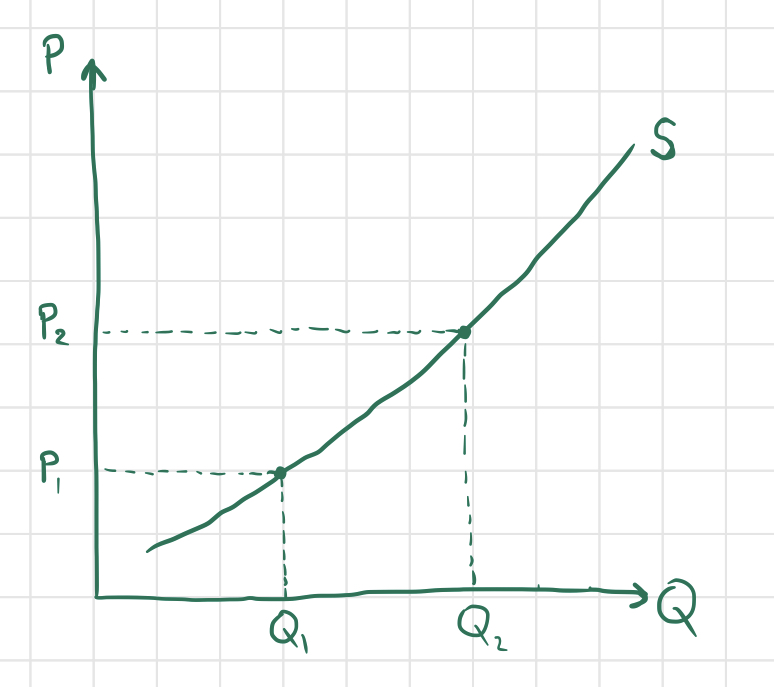
As explained above, firms will produce more of a good if the market price is higher, so the quantity supplied $Q_1$ at a lower price $P_1$ is lower than the quantity supplied $Q_2$ at a higher price of $P_2$.
So what determines the market price of a good? Of course, the market price of a good constantly fluctuates, but tends to settle on an equilibrium price determined by the supply and demand for the good. Let’s superimpose the supply and demand curves on a single graph and walk through the process of price determination:
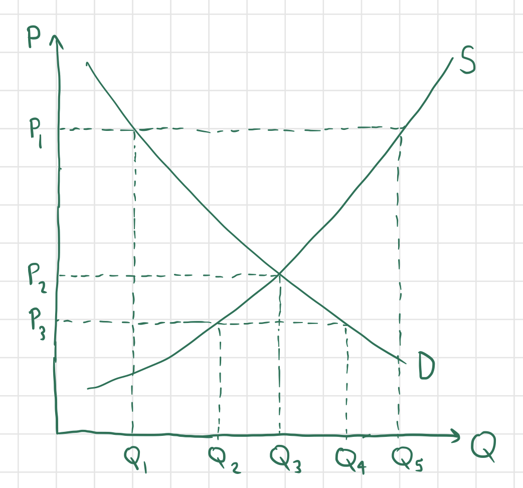
Consider the above graph, and suppose that the market price for good $X$ is currently at $P_1$. Then we can see that the quantity demanded by consumers will equal $Q_1$, while the quantity supplied by producers will be $Q_5$, which is greater than $Q_1$. This will lead to a surplus, since the quantity of good $X$ supplied is greater than than demanded; more specifically, $Q_5-Q_1$ units of good $X$ will be produced in excess. This is bad news for producers - customers aren’t buying all of the units of good $X$ that they are producing, so in order to entice more customers, firms will lower their prices, and the overall market price will lower.
Suppose instead that the market price for good $X$ is equal to $P_3$. Then the quantity supplied will be $Q_2$ and the quantity demanded will be $Q_4$. Since more good is demanded than is supplied, there is a shortage of good $X$, with $Q_4-Q_2$ more units of good $X$ needed. If firms notice that customers want more of good $X$, they will probably produce more of the good and raise their prices, since consumers are willing to pay more than they are currently paying for good $X$.
Finally, suppose that the market price for good $X$ is equal to $P_2$. In this case, the quantity supplied and quantity demanded are both equal to $Q_3$, incurring neither a shortage nor a surplus. At this price, consumers are happy because all of the consumers willing to buy good $X$ at price $P_2$ are able to do so, and producers are happy because they are selling all of the goods that they produce, but producing more and raising the price would result in a surplus. Thus, since this price is “stable,” it is the equilibrium price and the corresponding quantity supplied and demanded is called the equilibrium quantity. As explained above, if the market price for a good is above the equilibrium price, it tends to fall, and if it is below the equilibrium price, it tends to rise, so the market price for good $X$ will tend towards the equilibrium price $P_3$, at which the quantities supplied and demanded are equal (to $Q_3$).
The shape/slope of the supply and demand curves for a good vary based on the nature of the good. In particular, the elasticity of a good’s supply and demand curves reflect important properties of that good. The price elasticity of demand for a good at a particular price $P$ is defined at the percentage change in quantity demanded $Q$ per percentage change in price in a neighborhood of price $P$:
For example, if the price and quantity consumed of a good are $ $10$ and $20$ units respectively, and a price increase to $ $11$ results in a decrease in quantity demanded to $19$ units, we may approximate the price elasticity of demand as
If the price elasticity of demand is less than $1$, we say that the good in question has relatively inelastic demand, indicating that the quantity demanded of the good is relatively unresponsive to changes in price. If $E_d$ is greater than $1$, we say that the good has relatively elastic demand, meaning that the quantity of the good demanded responds more drastically to changes in price. If $E_d = 1$, we say that the good’s demand is unit elastic at the price in question.
For a more exact calculation of $E_d$, we may use calculus. If we are dealing with a continuous demand curve rather than discrete values of price and quantity demanded, we may express quantity demanded $Q$ as a function of price $P$:
If $f$ is differentiable, then we have
and
and so we have that
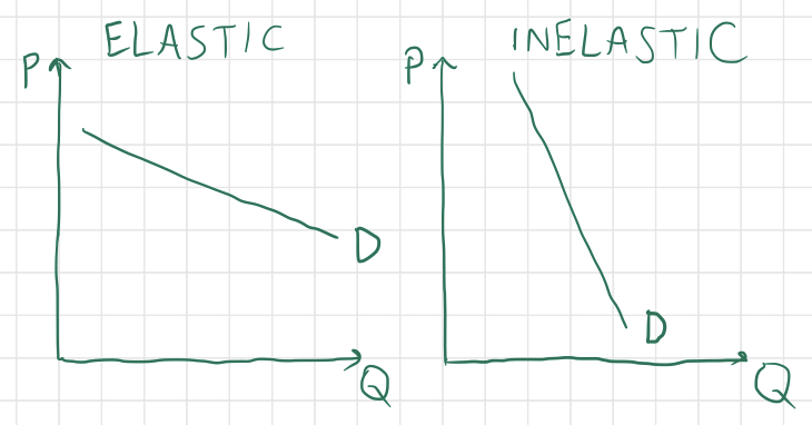
In general, steeper demand curves on the supply and demand graph indicate more elastic demand, while shallower demand curves are more inelastic. A demand curve that is perfectly elastic is simply a horizontal line, while a demand curve that is perfectly inelastic is a vertical line.
So what are some concrete examples of interpretations of elasticity of demand? Non-essential goods like chocolate or bicycles tend to have relatively elastic demand, since customers have no need to purchase them and most are willing to forego such goods if the price seems even slightly too high. However, goods like gasoline, medicine, and cigarettes have very inelastic demand, since most of the people who consume these goods are dependent on them, and cannot afford to give them up even if the price skyrockets (gasoline is needed to travel, medicine is required for some people to remedy urgent ailments, and cigarettes are addictive). The presence or absence of substitute goods also affects the elasticity of a good’s demand (more substitutes makes for a more elastic demand). For instance, if the price of chocolate doubles and the price of gummy bears stays constant, everyone except for the diehard chocolate-lovers with cash to spare will eat less chocolate and satisfy their sweet tooth with gummy bears instead. But if the price of gasoline doubles, everyone that drives a car will just have to tighten their belts and pay the price (unfortunately, cars can’t run on gummy bears).
Supply can be elastic or inelastic as well. If a good is very difficult to produce or start-up costs are very high for firms producing a particular good, then its supply is likely to be very inelastic (think uranium). Conversely, goods that are quick and easy to produce tend to have more elastic supply.
Various factors can affect the supply and demand of goods, so let‘s consider a few different scenarios and represent them using the supply-and-demand graphs that I‘ve showcased above. For each good and scenario described, try to guess what would happen to the price and quantity demanded for each good as a result.
Consider the market for bread, and suppose that it is fluctuating mildly around its equilibrium price and quantity of $P_1$ and $P_2$. Then, all of a sudden, a fungus overtakes the country‘s wheat crops, rendering most wheat unfit for human consumption. What happens to the supply, demand, price, and quantity consumed of bread?
The supply for bread would drastically decrease at each possible price, shifting the entire supply curve to the left (the demand for bread should remain unchanged, since people still want bread as much as they did before). Since suppliers can‘t produce as much bread in the absence of wheat (an input for the production of bread), the equilibrium quantity will surely decrease, and since bread becomes more scarce, the price will rise. The same result that we can reason out intuitively is illustrated on the graph below by shifting the supply curve to the left and observing the new point of intersection between the supply and demand curves:
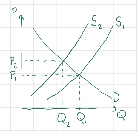
This type of situation is called a negative supply shock. There is also such thing as a positive supply shock, which might occur if, for example, scientists invented a new technology that quickly produces bread, or if a new strain of fast-growing wheat was discovered.
Here‘s another scenario. Consider the market for children‘s toys, and suppose that the propagation of a rumor causes consumers to believe that toy companies are using a toxic chemical to manufacture their toys. What happens to supply, demand, price, and quantity produced?
The supply remains constant this time, but the demand for children‘s toys will shift to the left since consumers don‘t want to buy as many toys, at any price. As a result, the price will fall (toy manufacturers have to lower their prices to entice customers) and the quantity demanded will also fall. Here‘s a graph:
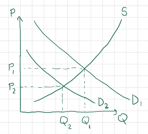
Actually, in the long run, the supply for toys could shift as well, since plummeting demand and prices for toys could drive some manufacturers out of business, bringing the supply down as well. But for now, we‘ll only consider the short-term effects of each scenario.
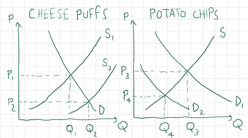
Okay, one more hypothetical situation. Consider now two separate markets - the market for cheese puffs and the market for potato chips. Suppose that researchers have discovered a fast and cost-effective way to convert discarded styrofoam into cheese puffs that are just as delicious (and addictive) as cheese puffs made with edible materials. Cheese puff manufacturers can now produce cheese puffs at a much lower cost, since they can use garbage plastic and styrofoam instead of more expensive biomaterials. What happens to both the markets for cheese puffs and potato chips?
Answer: for cheese puffs, supply and quantity increase and price decreases, and for potato chips, demand, quantity, and price all decrease. Since potato chips are a substitute for cheese puffs, as the price of cheese puffs decreases, lots of potato-chip-eaters will flock to cheese puffs as a cheaper alternative snack food. Here are two graphs representing the above situation:
If we were to consider the market for sour cream (or some other complement for potato chips), we would observe a decrease in demand there as well - if people buy less chips, then they will buy less of the things that go well with chips. The relationship between markets of substitute and complementary goods can be captured by the cross-price elasticity of a good $X$ with respect to good $Y$. This is defined as the percent change in quantity of good $X$ divided by the percent change in price of good $Y$ causing aforementioned change in quantity:
The sign of $E_{XY}$ suggests the relationship between $X$ and $Y$. In particular, if $E_{XY}$ is positive, it means that an increase in price of $Y$ causes a increase in quantity of $X$, implying that $X,Y$ are substitutes; conversely, if $E_{XY}$ is negative, it means that an increase in price of $Y$ causes a decrease in quantity of $X$, and so $X,Y$ are complements.
That concludes this introduction to supply-and-demand. In my next economics blog post, I plan to briefly describe a few other concepts relevant to supply and demand: consumer and producer surplus and deadweight loss.