The law of natural selection (or survival of the fittest) essentially states that in any environment, the organisms that are best suited to survive in that environment will survive and propagate, while those that are not will die off (as a result of competition with better equipped organisms, if not through any fault of their own). In the long run, this results in the formation of a semi-stable environment in which optimally-adapted organisms keep each other in check, and organisms’ genetic makeups reach an equilibrium. This is a slow process that occurs over the course of generations, so it is difficult for humans to study in real time. However, in recent years, computer scientists have been able to use the same process to “evolve” algorithms to complete tasks, which occurs much more quickly and can be observed in real time. To artificially replicate the process of natural selection, one must create a virtual “environment,” a population of “organisms,” and a method of assessing the organisms’ “fitness” in their environment. To mimic evolution and natural selection, computer scientists identify a task (like playing a virtual game, solving a puzzle, or something of that nature), randomly generate a population of algorithms for carrying out the task, have each individual attempt the task, assess the individuals, and eliminate poorly-performing individuals while keeping the top-performing individuals alive, and then repeat this process many times.
In this post, I will do something of this nature using Python. But before showing the code that I will use to simulate natural selection and evolution, I must outline a few of the key components of the program.
First of all, the individuals in the population need a task to complete. For my example, the task is as follows: each individual will play a game on a square grid with “white” and “black” squares. The individual will start on a white square and at any time may move to any adjacent square (up, down, left, or right), but moving onto any black square will end the game (“death”). Further, as the individual moves around the board, the white squares that it has formerly occupied will turn black, causing the individual to eventually run out of spaces to occupy. I will allow each individual to play the game a number of times, and use the average number of turns that the individual survives as a measure of its “fitness” or “competence.”
Then, after measuring the fitness of each individual in the population, I will sort the individuals based on their “fitness measure” and kill those in the bottom $50$ percent. Then the surviving organisms will “breed” to produce offspring. But let’s not forget the most important part - these offspring must experience low-probability mutations, allowing new and better strategies to evolve by chance.
Let’s get to the code. I’ll explain each part of my code, chunk by chunk, and then show the results of a few simulations. First, we have to import a few useful Python modules:
import itertools
import random
import matplotlib.pyplot as plt
import numpy as np
The itertools module contains some tools for iteration and loops, the random module allows the generation of (pseudo-) random numbers, the pyplot module will allow my to graph the results of my simulations on a scatter plot, and numpy contains a lot of standard mathematical functions.
The itertools module contains some tools for iteration and loops, the random module allows the generation of (pseudo-) random numbers, the pyplot module will allow my to graph the results of my simulations on a scatter plot, and numpy contains a lot of standard mathematical functions.
The first thing to do is create a way to virtually run the puzzle. To represent a two-dimensional board, we will use an array of arrays, like this:
This array would represent a $3\times 3$ grid. In the grid that we use, a zero will represent a white square, and a black square can be represented by any other character. We want to generate a board with black boundaries around the edges and randomly scattered black squares throughout (to add an element of randomness to the game). Here’s the code:
def gen_random_grid(dim_1,dim_2,prob,type='normal'):
    board = []
    board.append([1] * dim_1)
    for x in range(0, dim_2-2):
        if type == 'cylinder':
            row = [0]
        else:
            row = [1]
        for i in range(1, dim_1-1):
            if random.random() < prob and not [x,i] == [0,1]:
                row.append(1)
            else:
                row.append(0)
        if type == 'cylinder':
            row.append(0)
        else:
            row.append(1)
        board.append(row)
    board.append([1] * dim_1)
    return(board)
The arguments for this function are the two dimensions of the game board, the probability of any given white square to turn black, and an extra fourth argument whose value can either be ‘normal’ or ‘cylinder’ (‘normal’ is the default option, but using ‘cylinder’ will create a cylindrical board with no left and right boundaries). Also worth noting: I’ve made it so that the top-right-most square in the board cannot turn black, since I need to reserve at least one space for the players to start off on.
Just for convenience, here’s another function that prints out a game board in a readable way:
def display_grid(board):
    for x in board:
        print(x)
Let’s see what happens if we try to generate and display a 10 by 10 grid with a $1$ in $10$ chance of each white square turning black:
>>> display_grid(gen_random_grid(10,10,0.1))
[1, 1, 1, 1, 1, 1, 1, 1, 1, 1]
[1, 0, 1, 0, 1, 1, 0, 0, 0, 1]
[1, 0, 0, 0, 0, 0, 0, 0, 1, 1]
[1, 0, 0, 0, 1, 0, 0, 0, 1, 1]
[1, 0, 0, 0, 1, 0, 0, 0, 0, 1]
[1, 0, 0, 0, 0, 0, 0, 0, 0, 1]
[1, 1, 0, 0, 0, 0, 0, 0, 0, 1]
[1, 0, 1, 0, 0, 0, 0, 0, 0, 1]
[1, 0, 0, 0, 0, 1, 0, 0, 0, 1]
[1, 1, 1, 1, 1, 1, 1, 1, 1, 1]
Looks like it’s working as we intended. Now we need to come up with a way to generate players, so that each player contains a coded set of rules (“genes”) for traversing the board.
Here’s how we’ll do it. Each player will have a limited scope of vision, and will only be able to see the directly adjacent and diagonal squares, using those to decide what move to make next. Furthermore, players will have no memory about previous moves, because storing memory of all previous moves and possible decisions based on these moves for every single player would require a huge amount of storage.
When players observe the $8$ squares in their immediate vicinity (northwest, north, northeast, west, east, southwest, south, southeast), they will see that each of these squares is either black or white - that means that there are $2^8=256$ possible scenarios. Since each player can choose to move up, down, left, or right in response to each observation, the player’s “genome” will consist of a 256-element array of four characters (1,2,3,4, representing down, up, left, right respectively).
Another note: when I have players traverse the board and turn white squares to black where they previously stood, I’m going to replace the zeroes representing white squares not all with ones, but instead with numbers indicating the number of the move on which the player occupied that square. This way, when a player moves across the board, we can display the board afterwards and see the path that the player took.
When we initially generate players, their genome will consist of $256$ characters, chosen uniformly and at random from $[1,2,3,4]$. However, each player will also have a two-element array storing their location on the board as coordinates $[x,y]$, and an extra entry storing their score on the game. Here is a function randomly generating a new player:
def gen_random_player():
    genome = []
    for i in range(0,256):
        genome.append(random.randint(1,4))
    return([genome,[1,1],0])
The array titled ‘genome’ within the function is the 256-character gene sequence of the individual, the two-element array $[1,1]$ indicates that the player will start on square $[1,1]$ when starting a game, and the $0$ is there because the individual has yet to play any games. Now, here is a function that takes both a player and a game board as input, and simulates gameplay between them:
def play_game(player, board, readable=0):
    dim_1 = len(board[0])
    dim_2 = len(board[1])
    move = 0
    while board[player[1][1]][player[1][0]] == 0:
        player[2] += 1
        move += 1
        if player[1][0] == 0:
            sq_1 = board[player[1][1]-1][dim_1-1]
            sq_4 = board[player[1][1]][dim_1-1]
            sq_7 = board[player[1][1]+1][dim_1-1]
        else:
            sq_1 = board[player[1][1]-1][player[1][0]-1]
            sq_4 = board[player[1][1]][player[1][0]-1]
            sq_7 = board[player[1][1]+1][player[1][0]-1]
        if player[1][0] == dim_1-1:
            sq_3 = board[player[1][1]-1][0]
            sq_6 = board[player[1][1]][0]
            sq_9 = board[player[1][1]+1][0]
        else:
            sq_3 = board[player[1][1]-1][player[1][0]+1]
            sq_6 = board[player[1][1]][player[1][0]+1]
            sq_9 = board[player[1][1]+1][player[1][0]+1]
        sq_2 = board[player[1][1]+1][player[1][0]]
        sq_5 = board[player[1][1]][player[1][0]]
        sq_8 = board[player[1][1]-1][player[1][0]]
        action_index = terp(sq_1) + 2 * terp(sq_2) + 4 * terp(sq_3) + 8 * terp(sq_4) + 16 * terp(sq_6) + 32 * terp(sq_7) + 64 * terp(sq_8) + 128 * terp(sq_9)
        if player[0][action_index] == 1:
            player[1][1] += -1
            board[player[1][1] + 1][player[1][0]] = move
        if player[0][action_index] == 2:
            player[1][1] += 1
            board[player[1][1] - 1][player[1][0]] = move
        if player[0][action_index] == 3:
            player[1][0] += -1
            board[player[1][1]][player[1][0] + 1] = move
        if player[0][action_index] == 4:
            player[1][0] += 1
            board[player[1][1]][player[1][0] - 1] = move
        if player[1][0] < 0:
            player[1][0] += dim_1
        if player[1][0] > dim_1 - 1:
            player[1][0] += -dim_1
    player[1] = [1,1]
    if readable == 1:
        display_grid(board)
    return(move)
I will admit that this is a gross function, and there’s probably a way to clean it up so that it will work more efficiently. The reason it’s so long and redundant-seeming is that a lot of casework has to be done to allow the player to view the immediately adjacent and diagonal squares on the game board and map each scenario to the appropriate move in its gene sequence, and then make the move (and possibly wrap around to the other side of the board, if it is cylindrical). I’ve also attached an optional parameter to make the board “readable,” so that the board is printed out after the simulation occurs.
So let’s test out what we have so far by generating a random player and having it play on a randomly generated $10\times 10$ grid:
>>> play_game(gen_random_player(),gen_random_grid(10,10,0.1),1)
[1, 1, 1, 1, 1, 1, 1, 1, 1, 1]
[1, 1, 2, 0, 0, 0, 1, 0, 0, 1]
[1, 0, 3, 1, 0, 0, 1, 0, 0, 1]
[1, 0, 1, 0, 0, 1, 0, 0, 0, 1]
[1, 0, 0, 0, 0, 0, 0, 0, 0, 1]
[1, 0, 0, 0, 0, 0, 0, 0, 0, 1]
[1, 0, 0, 0, 0, 0, 0, 0, 0, 1]
[1, 0, 0, 1, 0, 0, 0, 0, 0, 1]
[1, 0, 1, 0, 0, 0, 0, 0, 0, 1]
[1, 1, 1, 1, 1, 1, 1, 1, 1, 1]
3
Clearly, the player didn’t fare so well. It lasted for only three moves, walking idiotically right into a black square when there were plenty of white squares in the neighborhood. But we shouldn’t really have expected much from this player - after all, its gene sequence was completely randomly generated. To get some smarter players, we have to implement natural selection.
First, here’s a function to generate a random population of players of a given size:
def gen_player_array(n):
    population = []
    for i in range(0, n):
        population.append(gen_random_player())
    return(population)
And here is a function that randomly mutates a player’s gene sequence, altering each character with a specified probability:
def mutate_player(player, prob):
    for x in player[0]:
        if random.random() < prob:
            x = random.randint(1,4)
    return(player)
Next, a function that takes an array of players (that have already played the game multiple times) as an argument and sorts them based on their score:
def sort_by_scores(player_array):
    sorted_players = []
    for j in range(0,len(player_array)):
        top_player = [0,0,0]
        top_player_index = 0
        for i in range(0, len(player_array)):
            if player_array[i][2] >= top_player[2]:
                top_player = player_array[i]
                top_player_index = i
        sorted_players.append(top_player)
        del player_array[top_player_index]
    return(sorted_players)
Finally, here’s a function that takes as input a population of players already sorted by fitness, kills off the bottom half, and allows the top half to “breed”:
def evolve_sorted_players(player_array, prob):
    for i in range(0, int(len(player_array)/2)):
        player_array[i][2] = 0
        child = [[],[1,1],0]
        for j in range(0,256):
            if random.random()<0.5:
                child[0].append(player_array[0][0][j])
            else:
                child[0].append(player_array[i][0][j])
            if random.random()<prob:
                child[0][j] = random.randint(1,4)
        player_array[i + int(len(player_array)/2)] = child
This one requires a bit more explanation, because of the particular way in which the players breed. When two players breed, the child’s gene sequence is formed by choosing for each entry either one parent’s entry at the same index or the other’s, with equal probability. Then, after forming the child’s gene sequence by weaving together parent sequences, the function applies the random mutation function to the child. So after it kills the bottom half of players, this function allows the single top-scoring player to breed once with each other player in the top half, replacing the killed players and keeping the population stable. Yes, the top-player also “mates” with itself, but don’t worry, these creatures bear no real resemblance to any organisms in real life, so nothing nasty is happening here.
Okay, there’s only one more big function that we have to set up, and then we’ll be ready to run some simulations. Here it is:
def generations(population, num_rounds, gens, mutate_prob, no_ice_prob, sample_players=0, sample_interval=0):
    pop = gen_player_array(population)
    top_score = []
    av_score = []
    bot_score =[]
    gen = range(0,gens)
    sample_ticker = 0
    samples = []
    for i in gen:
        sample_ticker += 1
        for p in pop:
            for x in range(0,num_rounds):
                play_game(p, gen_random_grid(10,10,no_ice_prob))
            p[2] = p[2]/num_rounds
        pop = sort_by_scores(pop)
        top_score.append(pop[0][2])
        bot_score.append(pop[-1][2])
        av_score.append(sum([x[2] for x in pop])/len(pop))
        evolve_sorted_players(pop, mutate_prob)
        if sample_players == 1 and sample_ticker == sample_interval:
            sample_ticker = 0
            samples.append(pop[0])
    plt.scatter(gen, top_score, color='g')
    plt.scatter(gen, bot_score, color='r')
    plt.scatter(gen, av_score, color='b')
    plt.title('pop = ' + str(population) + ', rounds = ' + str(num_rounds) + ', gens = ' + str(gens) + ', mutation prob = ' + str(mutate_prob) + ', black prob = ' + str(no_ice_prob))
    plt.show()
    plt.clf()
    if sample_players == 1:
        return(samples)
Using all of the functions we’ve defined so far, this function randomly generates a population of a specified size, allows each player to play the game a specified number of times (and the probability of black squares appearing across the board is a modifiable parameter), sorts them based on their average scores, allows natural selection to occur (the mutation probability is also a modifiable parameter), and then repeats the process for a certain number of generations. At each generation, it also keeps track of the top, bottom, and average scores of the population, so that we can plot and analyze this data after the simulation is run. There are also two optional parameters labelled ‘sample_players’ and ‘sample_interval,’ which allow us to instruct the program to stop simulating after a certain number of generations and extract a “sample” by appending the top player to an array and returning the array at the end. This way, after running the simulation, we can get a taste of the individual behaviors of the top-performing players throughout the simulation.
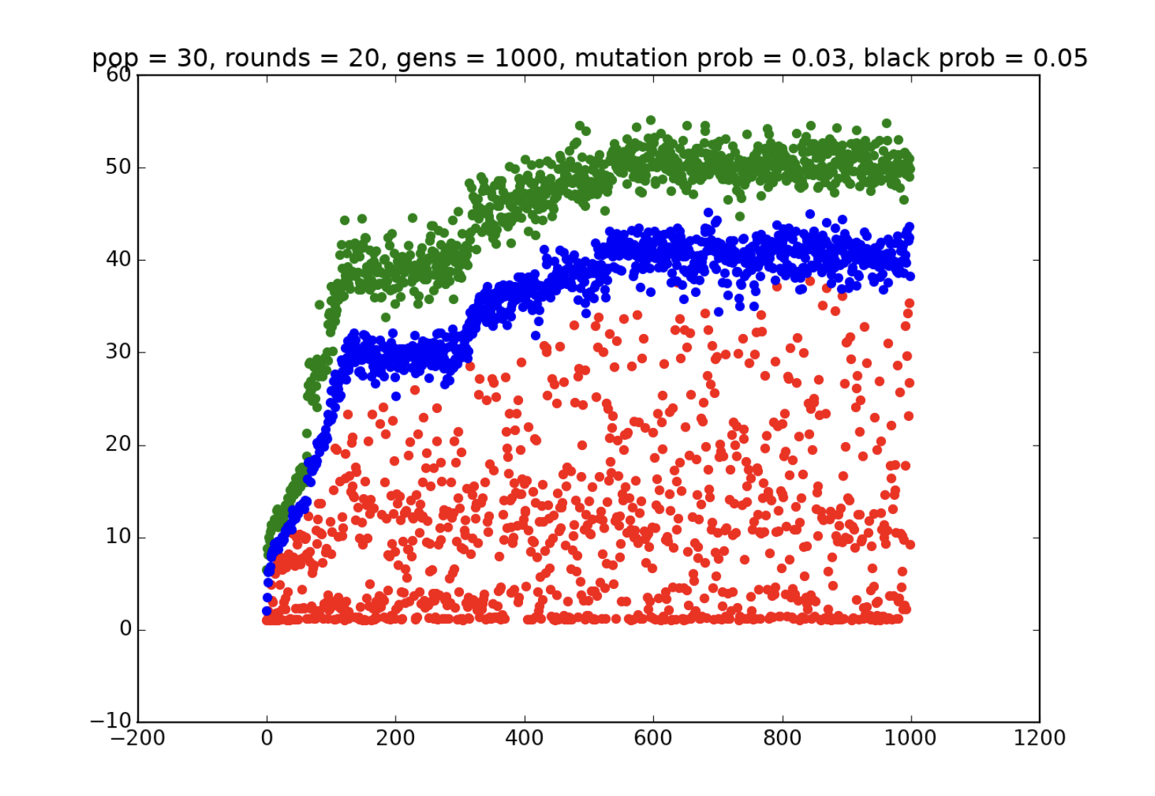
Great! Now let’s simulate! To start off, let’s try a simulation with 30 players, 20 games played per player, 1000 generations, probability 0.05 of white squares turning black, and mutation probability 0.03. To do this, we must run the command
>>> generations(30,20,1000,0.03,0.05)
Doing this outputs the following graph of player performance over the course of the generations:
Each green point represents the score of a top-performing player during a generation, each blue point represents the average score of all players in a generation, and each red point represents the lowest score in a generation. We can notice a few significant things from this graph right away. First of all, the top score seems to be (more or less) increasing the entire time, which confirms our expectations that natural selection fosters a fitter population. However, this increase isn’t exactly uniform over the course of the experiment. Performance seems to increase very quickly at first, until somewhere between generations 100 and 150, where it temporarily levels off. Then, around generation 250, it begins increasing again, until it levels off at an optimal average score of about 40 and an optimal top score of about 50. Why do we have this “staircase effect,” where the gene pool increases, levels off, and then increases again? Why isn’t there a steady increase during the entire experiment?
Before we move on, this graph hints at another interesting phenomenon that is easier to explain. While the top and average scores clearly increase over the course of the generations, the bottom score shows very little improvement and appears more or less random (but is more often much lower than both the top and average scores). After many generations have passed, the consistently poorly-performing individuals should already have been killed off, meaning that the poorly-performing individuals that appear in later generations are probably recently born, suggesting that their failure is a result of some sort of “breeding error.” This could be because it receives genes from two parents with incompatible genes, or because a random mutation messed up some important “adaptation” that it inherited from its parents. And it is indeed the case that running simulations with varied mutation probability values shows that higher mutation probabilities lead to the lowest scores being clustered at the bottom and lower mutation probabilities lead to more evenly spread and higher lowest scores (though I will not show these simulations here; copy the code and try it out for yourself if you like).
To get a better idea of what’s going on here, let’s run another simulation, this time storing the top-scoring player of every 50th generation in an array (called sample_player_arr) so that we can examine these strategies after seeing the graph.
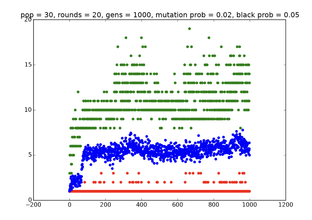
sample_player_arr = generations(30,20,1000,0.02,0.05,1,50)
Here is the graph produced:
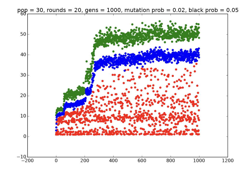
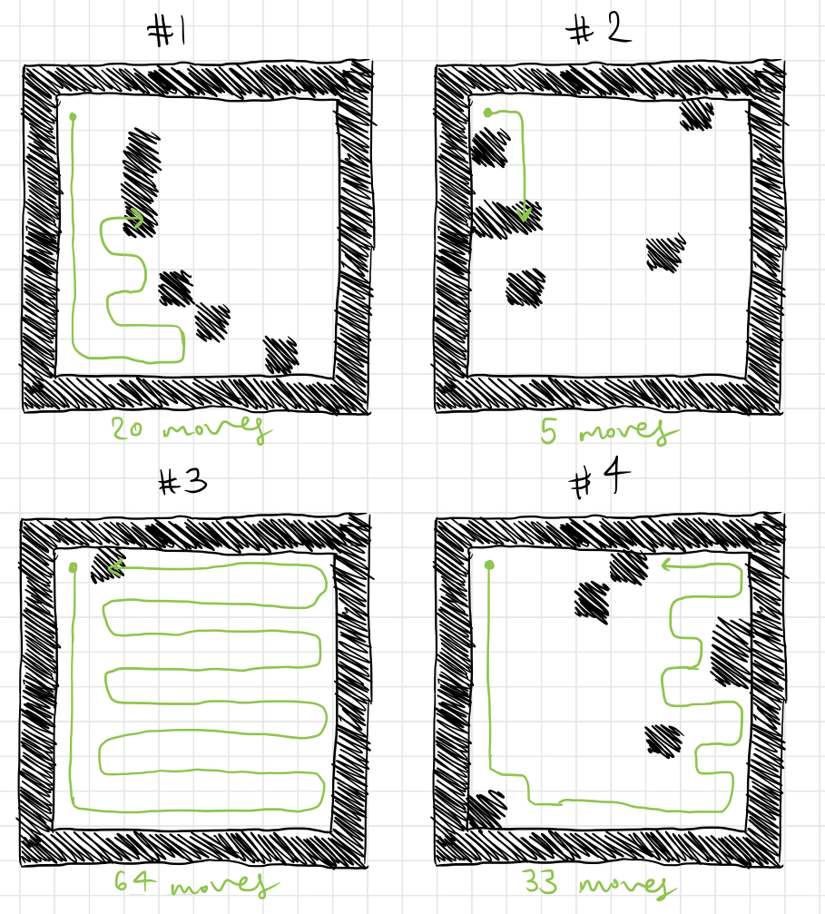
The rough stair-steps are also present here, with a short one from around generation 30 to generation 50, two more short plateaus from generations 150 to 200 and 200 to 250, separated by a brief increase, and a sharp increase around generation 250 before finally leveling off. Now let’s see these players in action! We’ll start by taking the top-player from generation 50 and making it play a few games on a random board. Instead of showing the code, I’ve drawn out the results of a few games in a way that is easier to see:
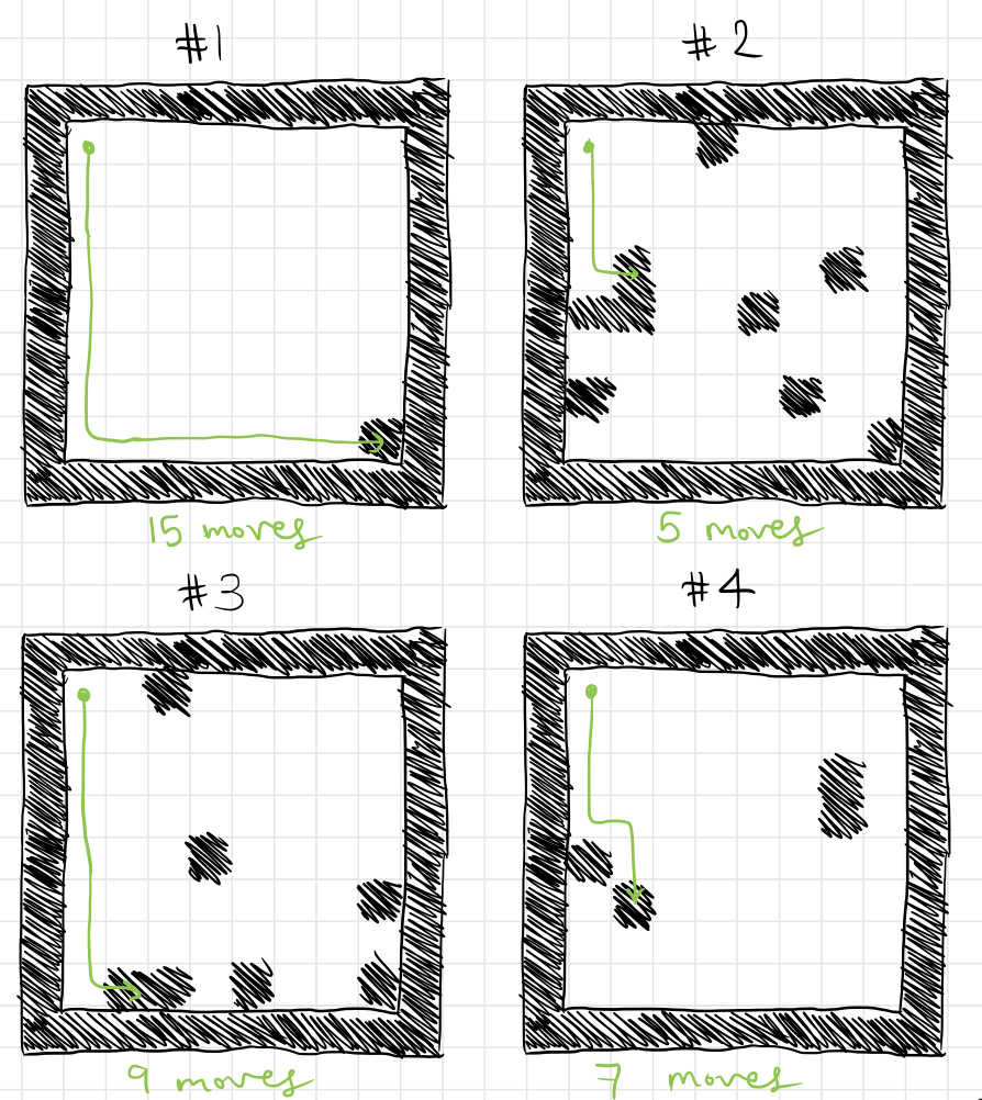
While these games aren’t exactly optimal, we can clearly see that the player isn’t just staggering about randomly. Its movement is definitely systematic, although it might not be quite as “smart” as a strategy designed explicitly by a human.
If we were to purposefully design a strategy, the first thing we would do is teach it not to walk into black squares and prematurely end the game if there is a white square in the vicinity (that is, don’t die unless trapped). However, this population seems not to have learned this yet, as it makes “stupid” mistakes almost immediately by walking onto black squares in games 1 and 4 even though there were adjacent white squares available.
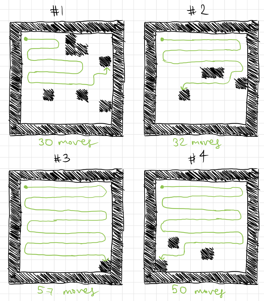
Here are some games played by the top player from generation 150:
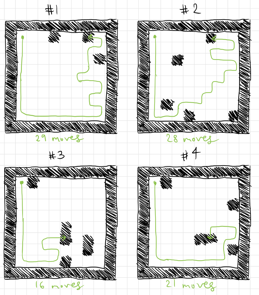
This strategy performs consistently better than the one from generation 50, and it clearly commits fewer avoidable errors, allowing it to survive longer, but still two of these deaths could have been avoided by walking onto an adjacent white square instead of a black one. While some of the previous strategy’s flaws have been fixed, some still remain, either because they were never “fixed,” or because they were messed up by random mutation.
Here are four games played by the top player from generation 400, during the final plateau of the simulation:
Once again, two of these deaths resulted from avoidable mistakes (in game 1, for instance, the player easily could have proceeded upwards instead of to the right in order to avoid dying). However, the player still avoids many more mistakes that players from earlier generations committed.
It’s worth noting that the simulation explored in detail above is not necessarily representative of all possible outcomes of the system. In some other simulations carried out afterwards, I noticed that the stair-stepping effect sometimes turned out to be more or less clear. Furthermore, the strategy evolved often turns out to be a little bit different, sometimes forming a horizontal zigzag, or even a spiral.
Now would also be a good time to discuss the effect of the particular scoring mechanism that we put in place. By using the players’ average score to rank them, we placed no value on consistency or reliability, which is reflected in some of the examples above. In other words, players that do fairly well most of the time would receive the same ranking (or a lower ranking) than players that do poorly most of the time and very well on occasion, since the occasional excellent scores would make up for the frequent failures. This is reflected, for example, in the player from generation 400 receiving the drastically different scores of 5 and 64 on two consecutive games - if players were ranked based on their minimum score, such a player would have received only an aggregate score of 5.
In fact, to see what would happen, I tweaked my code to instead rank players based on their minimum score received over the course of a certain number of games, rather than their average score. The result was rather interesting - the players perform well much more consistently than the players generated by the previous experiment. Here’s a graph for a simulation that I ran in which players were evaluated instead based on their minimum scores:
This may not look very impressive, but keep in mind that this is a graph of the top player’s minimum score, the average minimum score, and the bottom player’s minimum score from each generation. In that respect, it is much more impressive than the strategies generated by the previous simulation, which often played a few spectacular games and failed miserably on the rest. Here are a few test games with the top player from generation 1000:
That should serve as an adequate demonstration that the measurement used to rank members of the population has a great effect on their performance. It isn’t just as simple as selecting for the “best” players; their performance depends heavily on how we choose to define “best.”
I’ll conclude this post with a short list of factors that influence the outcome of these simulations, and the types of traits that members of the population evolve. Some of these factors haven’t been discussed in depth in this post, but I have done a bit of experimentation with them on my own.
I’d like to repeat this experiment in a future blog post, perhaps in a more thorough and rigorous way, and with a different task/puzzle for players to complete. I would encourage any interested reader to copy the code outlined in this post and experiment with it independently.