In this blog post, I’ll explore how (virtual) organisms evolved to succeed in a particular environment are affected by a change of environment. To do this, I’ll use a genetic algorithm (GA) similar to the one I used for my AP Research project. My research paper contains a thorough explanation of what genetic algorithms are and how they work, so if you’re unfamiliar with GAs, I suggest you read the first two sections of my research paper linked above (Melanie Mitchell’s book Complexity also contains a nice intro to GAs, from which I’ve stolen the “soda can collection problem” used below). Everything in this post meant to be accessible to any reader with a bit of background knowledge about GAs.
Despite the many practical applications of genetic algorithms, my GA will be dedicated to solving a simply and wholly impractical “toy problem” used by Melanie Mitchell in her book Complexity. Why? Because the purpose of this blog post is not to solve a particular problem, but to explore and gain an intuition about how the environment in which an organism evolves (real or virtual) affects its performance in other environments. By using a variant of Mitchell’s simple and easy-to-visualize “soda can collection problem,” we ensure that the results of the GA will be easier for us to intuitively grasp. However, it’s worth recognizing that whatever intuitive discoveries we make here may not be applicable to other genetic algorithms, not to mention real evolved living organisms - the simplicity of the problem (and its total lack of resemblance to an organic biological system) will fundamentally limit the scope of our results. I hope, however, that the experiment will nevertheless be interesting and elucidating.
Here’s a description of how the problem works:
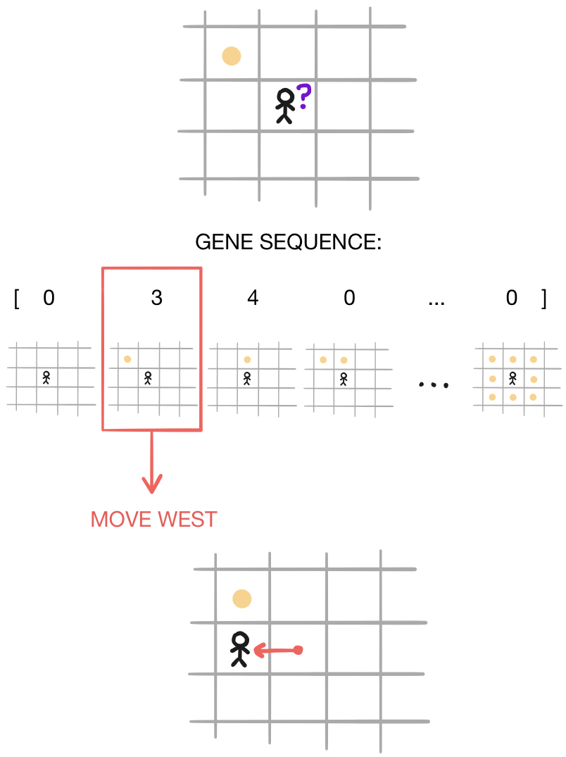
Each player has a “gene sequence” of $256$ characters, each of which is either $0,1,2,3,$ or $4$. These characters correspond to five different possible actions the player may take: move north, move south, move east, move west, or move in a random direction. Before making a move, the player first “observes” the $8$ squares horizontally, vertically, and diagonally adjacent to it. Since each of these squares can be in one of two states (either empty or containing a token), there are $256$ different possible states that the player could observe. Each of these states corresponds to a certain position in the player’s gene sequence. In order to decide how to move, the player looks up the character in its gene sequence corresponding to the situation it is currently in, and makes the move indicated by that character.
Keep in mind that when these “players” play the game, it’s much different that if you or I were to try playing this game, for a few reasons:
So if you aren’t impressed by the solutions yielded by our genetic algorithm, keep these points in mind. Also, remember that our purpose is not to develop phenomenal solutions to the “soda-can collection problem,” but to gain insights about genetic algorithms.
We have just a few more formalities to discuss before getting to the fun part. Before moving on, I’d like to identify a few parameters that can be tweaked to yield slightly different versions of our problem or genetic algorithm. By changing the values of these parameters, we can create “different environments” to evolve players in:
There are a few other parameters, but they alter the structure of the genetic algorithm rather than the problem being solved by players:
There are two main ways that we’ll be viewing data over the course of this blog post. One easy way of viewing data is with graphs, and I’ve generated two types of graphs to help us visualize data over the course of this post. We’ll refer to the first type as a generational proficiency graph that shows how the fitness values of players in the population change from generation to generation. They usually look something like this:
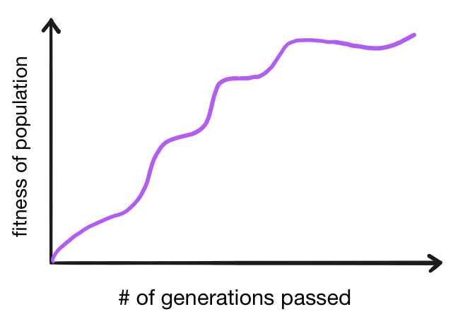
As generation after generation goes by, the overall fitness of the population increases as poorly-performing individuals are weeded out and more proficient ones “reproduce” with each other. Note that it is not impossible for fitness to occasionally decrease from one generation to the next - the simulation contains a great degree of randomness, so a series of debilitating mutations could cause a particular population to perform poorly by chance. Also, notice that the “fitness of population” measurement on the y-axis is a bit ambiguous, as we could measure a population’s overall fitness in a number of ways, such as the average fitness of players in the population or the fitness of the highest-performing player in the population. In this post, we will use the latter. Here’s an example of a generational proficiency graph made with data from an actual simulation:

The second type of graph will be called an environmental crossfitness graph. It shows how the fitness of a population of players changes based on its environment, and may look something like this (although, as we will see later, they can look very different):
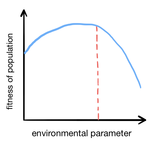
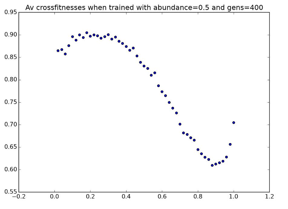
All environmental parameters are held constant, except for a single parameter (such as token abundance, for example), which is varied along the x-axis. A population is trained in an environment with a fixed value of this parameter (indicated by the dashed red line), and this population’s fitness is then tested in environments for which it was not trained. For example, we might raise a population of players in an environment with $p=0.5$, in which tokens are moderately abundant. Then we could allow these same players to play in environments in which tokens are very scarce ($p=0.1$) or very abundant ($p=0.9$) to see how they perform in unfamiliar environments. In the simplified graph above, the players perform best in the environment that they were raised in, as we might expect - but the graph below, created with real data for a population raised in the condition $p=0.5$, shows that this is not always the case:
Another method we will use to understand our data is viewing animations of actual players playing the game. This will allow us to qualitatively observe the strategies they use, and how these strategies change depending on the environment that the player adapts to. Here is a first-generation player (with an entirely random genome) playing the game with $r=c=10$, $a=0.5$, and $l=100$:
Not very impressive - that’s what we should expect from a player with random instructions. Contrast that with this animation of a player from the four-hundredth generation of a genetic algorithm raising players in an environment with $r=c=10$, $a=0.5$, and $l=100$:
Still not perfect, but much better! These animations are pretty helpful for visualizing what’s actually going on when players’ fitness increases over the course of a GA’s generations.
Before we continue, I’d like to make a little disclaimer: none of what I’m doing in this post is rigorous research. In my research project, I took precautions (like large sample sizes and consideration of statistical significance) to make sure that my claims were supported, and qualified all of my intuitive explanations. This post, however, will involve a lot of speculation and non-rigorous observation derived from isolated simulations, not large sample sizes.
To see how the abundance of tokens in players’ environment affects their fitness, we must hold all environmental variables constant. In this section, we’ll consider a range of different values for $a$, the token abundance, while keeping the other parameters constant at $r=c=10$ and $l=100$.
When we use environmental crossfitness graphs in this section, we have to be careful about how we measure “population fitness” and “player fitness.” To see why, consider the following question. Which of the following players would you say is better adapted to its environment?
We may be tempted to say that the second player is “more fit” because it collects more tokens per game on average. However, the second player also has access to more resources, since it lives in an environment with a higher token abundance - so player two has an advantage just because of its environment, not because of any effective strategy it uses. When player one plays the game, its game board only contains $0.2\cdot 100=20$ tokens on average, while player two usually plays on game board with about $0.9\cdot 100=90$ tokens. This means that player one collects about $18/20=90\%$ of the available tokens per game, while player two collects about $54/90=60\%$ of the available tokens per game, suggesting that player one is more fit. This seems like a “fairer” method of comparing the scores of players in different environments. To account for this, on the y-axes of our later environmental crossfitness graphs, “population fitness” is not calculated by averaging players’ scores across the population, but by averaging the following statistic across all players in the population:
In other words, population fitness is calculated by averaging the proportion of available tokens that each player collects.
Let’s begin by looking at an environmental crossfitness graph for a population of players evolved in environments in which tokens are scarce. The following three graphs are environmental crossfitness graphs for populations of players trained on game boards with $a=0.1$, $a=0.2$ and $a=0.3$ respectively:
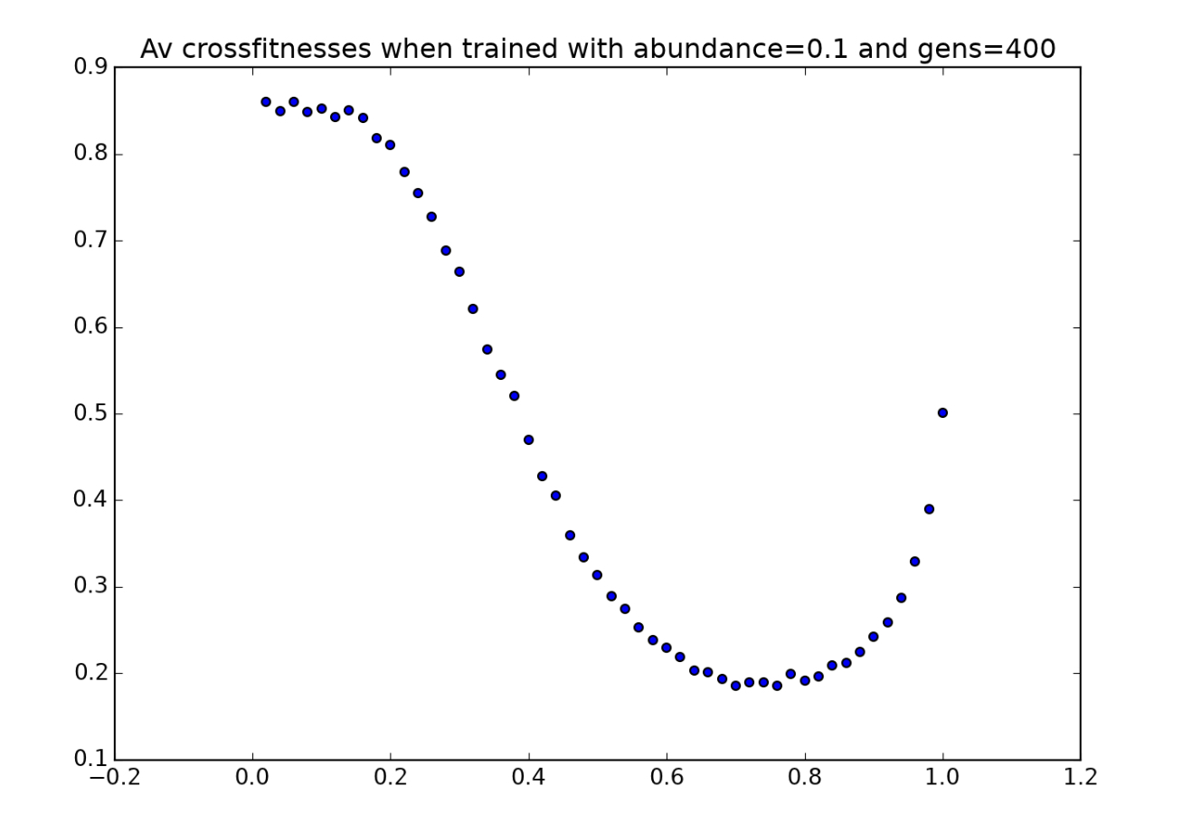
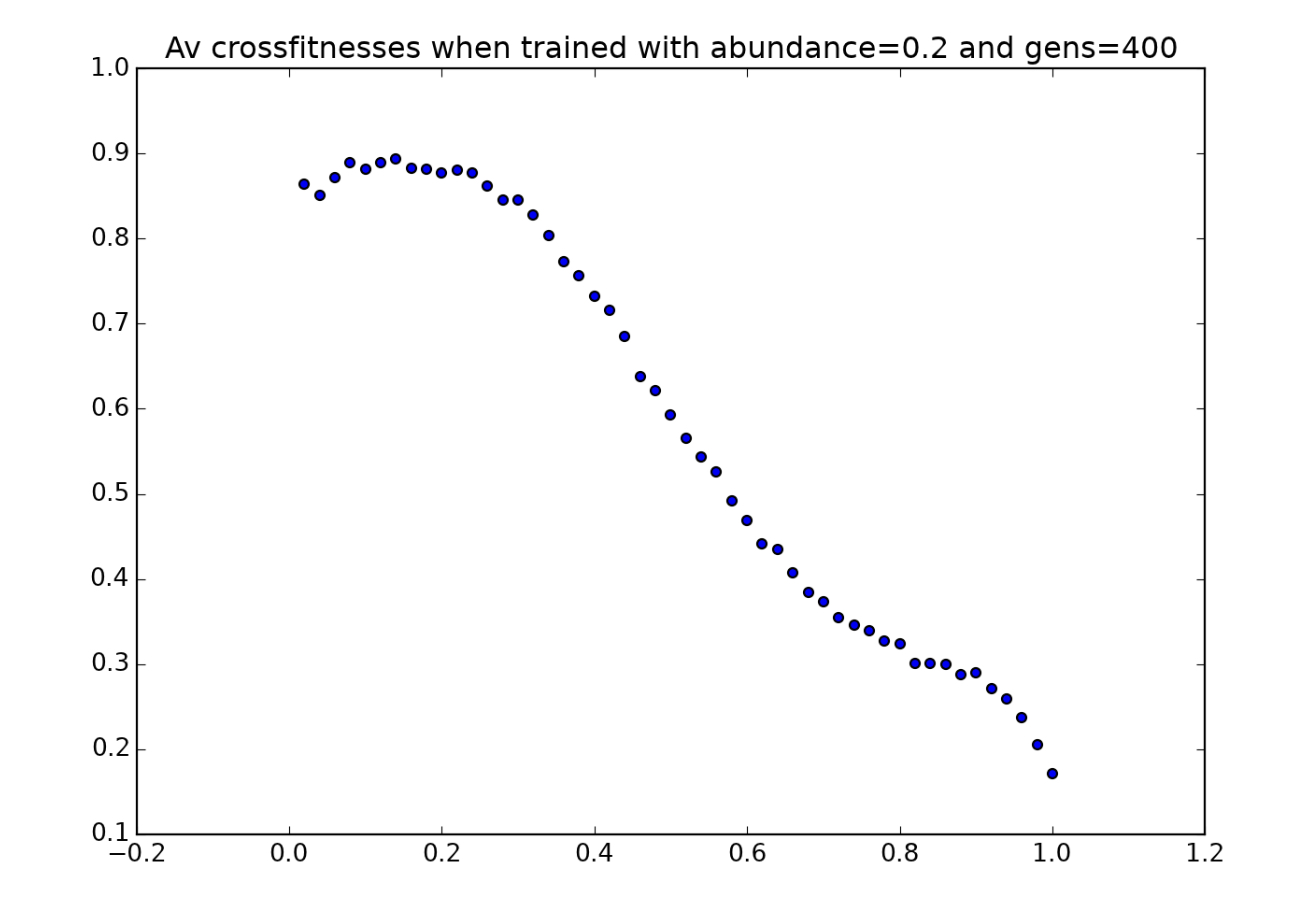
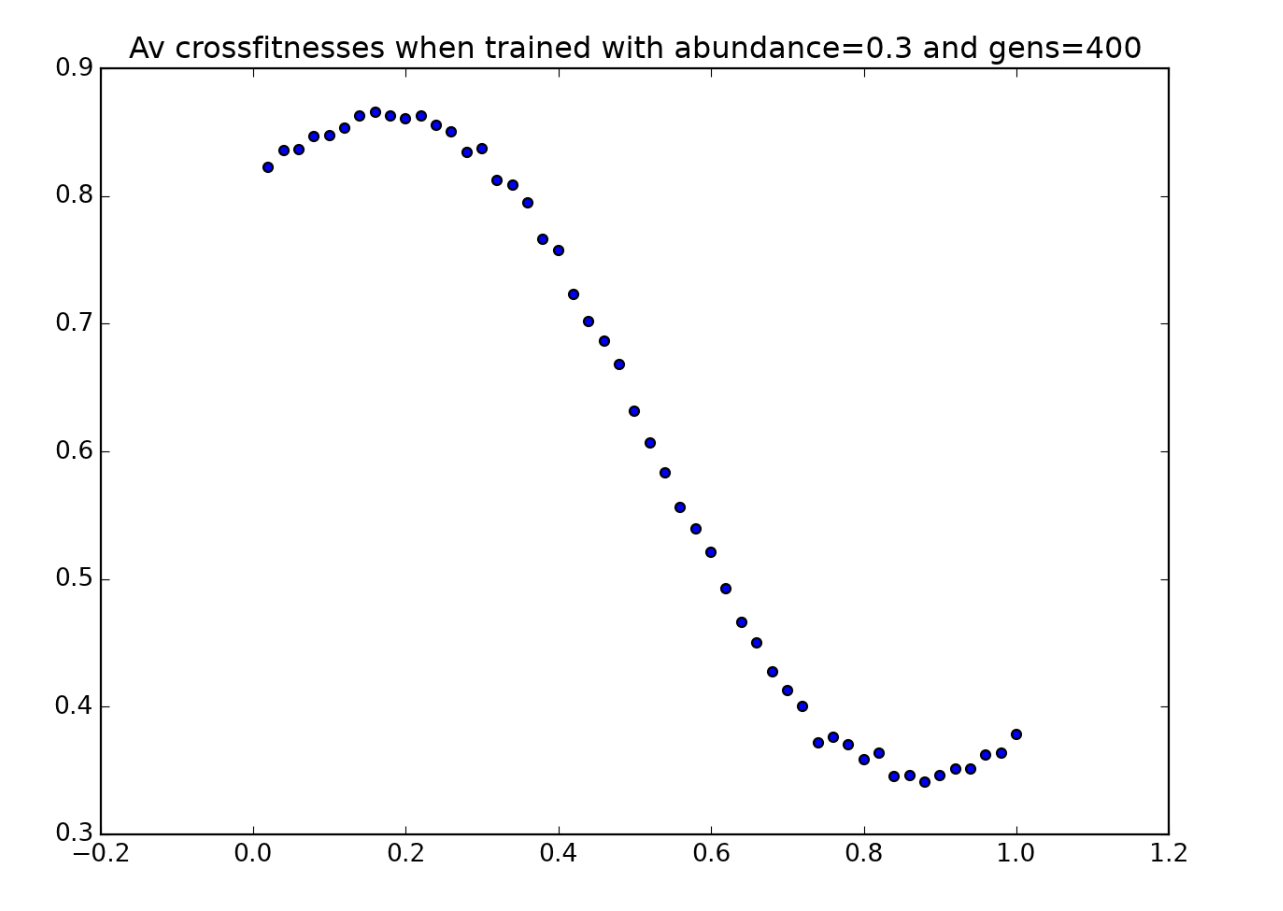
Here are a couple noteworthy observations:
Now let’s take a closer look at what’s going on by observing some individual games with players in these sample populations. Here are three players (from environments with $a=0.1,0.2,0.3$ respectively) playing in their “native habitats.” Watch how they behave and move around the board, and try to notice some features of their strategies.
These animations make two interesting aspects of these players’ strategies apparent:
Let’s consider this second point for a moment and think about why a greedy strategy might not always be optimal. Here’s an example of an sequence of moves made by the players in both the first and third animations that might seem sub-optimal, and certainly aren’t greedy:
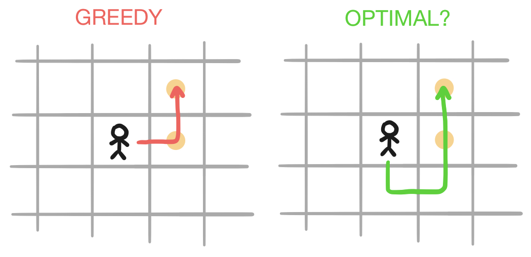
It’s possible that this behavior is the result of a random mutation, so we can’t draw any definitive conclusions from it. However, I do have a tentative explanation for why the second option might be more optimal. Consider the following scenario in which there are three tokens, rather than just two as in the scenarios above:
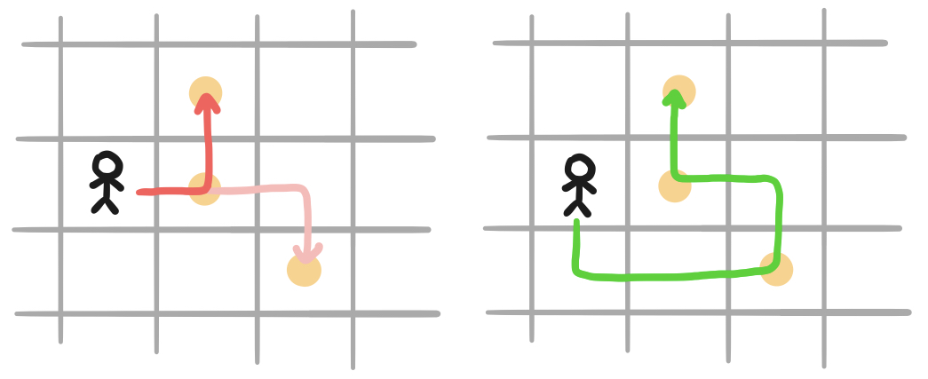
If a player behaves greedily in this situation, after collecting the token in the center, it must choose between the northern and southeastern tokens. Once the greedy player has taken the center token, it can’t get to both of the two remaining tokens because they’re not visible from each other - remember that the player has no memory of previous moves, so once the player proceeds north to collect the northern token, it forgets that the third token exists. The odd behavior observed in our animations would solve this problem. By taking a short detour (costing it a few extra moves), it is able to collect all three tokens in one swoop. This strategy might not always pay off, since there may not always be a third token in this position. However, in token-scarce environments, it makes sense that players would want to avoid having to leave any tokens behind.
So far we’ve just watched these players perform in their native environments. Now let’s see how they do in environments that are more token-abundant. Below are animations of the same three players playing in environments with $a=0.6$:
Ouch! To be honest, the second player does fairly well, but the fact that the first and third players end up like dogs chasing their tails suggests that this may be a fluke. A greedy strategy might have served these players better in this environment - despite the second player’s decent performance, we can see how all three players acting “too careful” in a token-abundant environment caused them to waste a lot of time.
There’s another good evolutionary reason why these players are more likely to make “stupid mistakes” when they are surrounded by many tokens. Players in token-scarce environments hardly ever find themselves surrounded by four or more tokens at a time, so the characters in their gene sequences coding for those scenarios are probably hardly ever used. This means that there is very little evolutionary pressure on those parts of their gene sequence. A population of players could evolve to be great at coping with a low-abundance environment without ever improving the subset of their genes that codes for high-abundance scenarios, because those genes aren’t used very often and therefore aren’t selected for.
Now let’s look at some populations of players raised in environments with moderate and high token abundance. For the sake of brevity, I won’t dissect these examples as thoroughly as I did the previous ones.
Here are three more environmental crossfitness graphs, corresponding to players raised in environments with $a=0.4,0.5,$ and $0.6$:
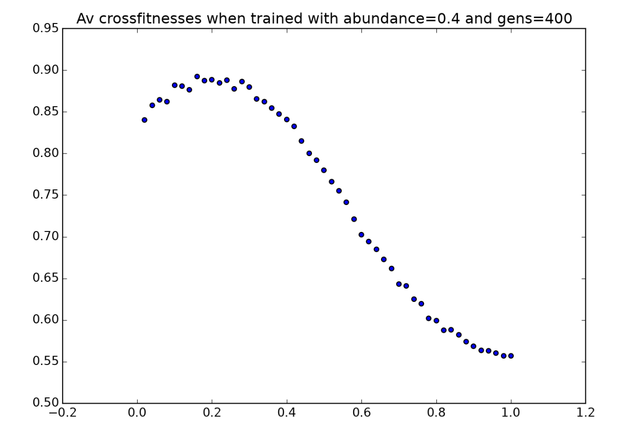
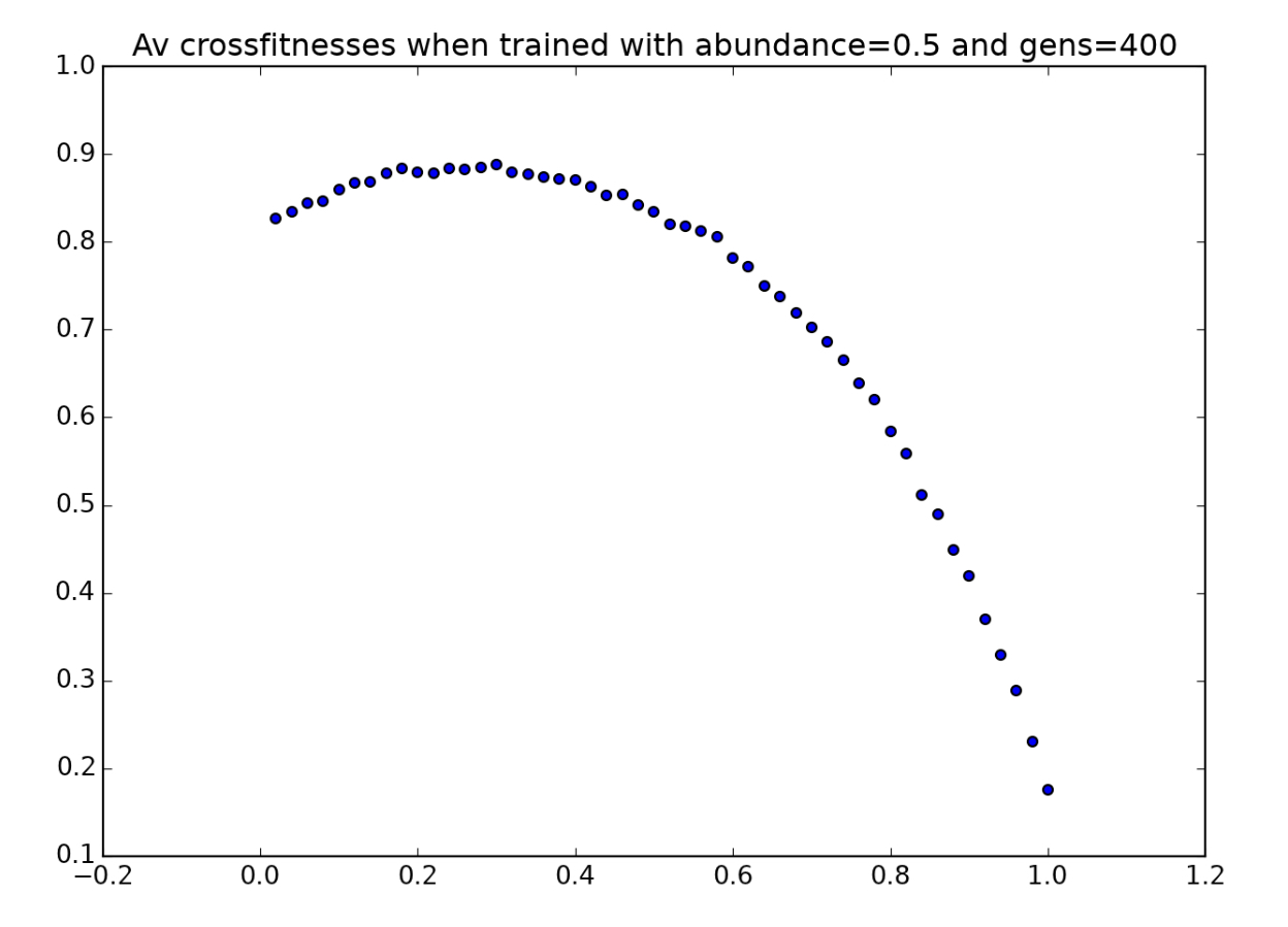
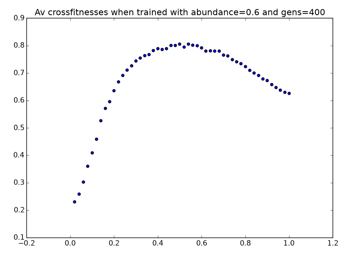
And here are three sample players, one for each different token-abundance value, playing in their “native habitats”:
For the most part, these are similar to the low-abundance examples we saw, and the animations show us some of the same techniques we observed before. However, in the third animation, a new strategy appears: when the player doesn’t see any tokens in its environment, rather than moving in a random direction, it moves exclusively in one direction. This strategy does cost the player some tokens at the end when it gets stuck going in a loop, and it could be the result of a mutation. However, given that this player was the highest-performing in its population, it’s probably a feature rather than a bug.
This is further supported by the fact that this same strategy is also used by players trained with $a=0.7,0.8,$ and $0.9$. Here are the environmental crossfitness graphs for players trained for those a-values:
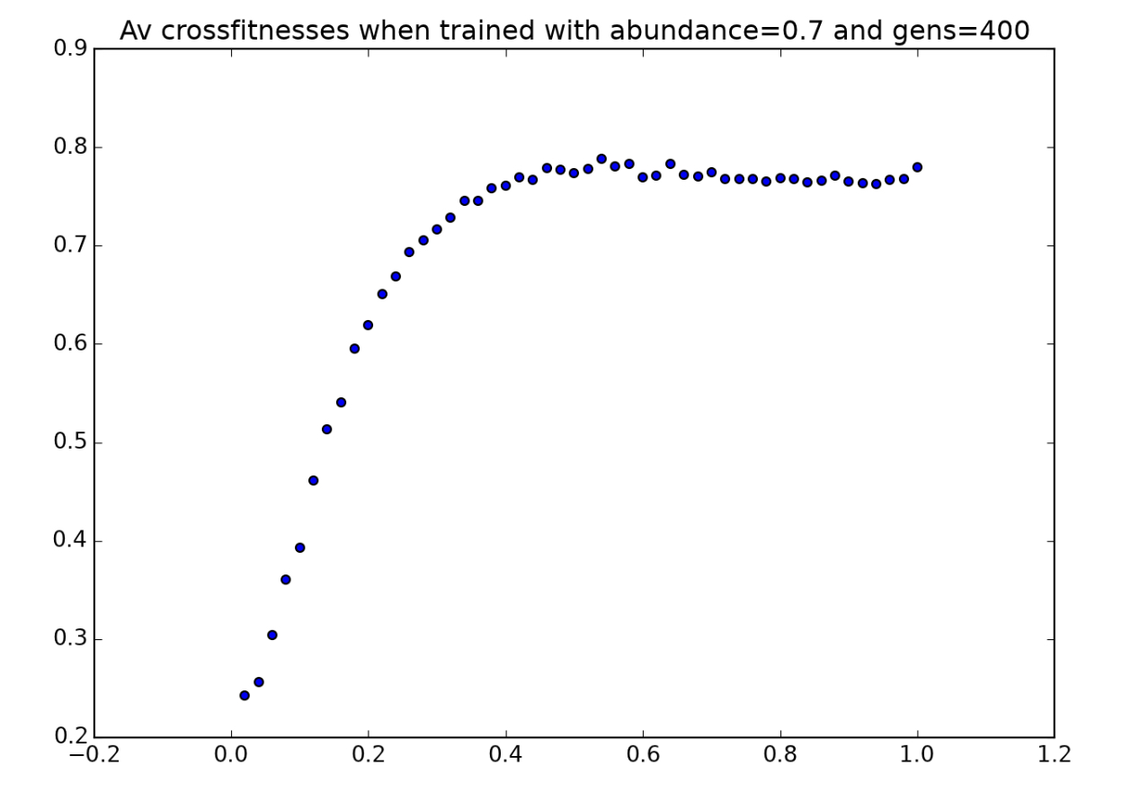
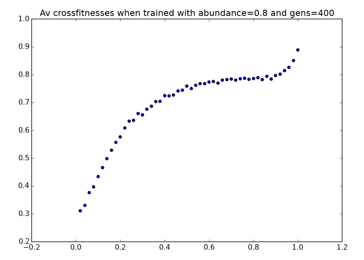
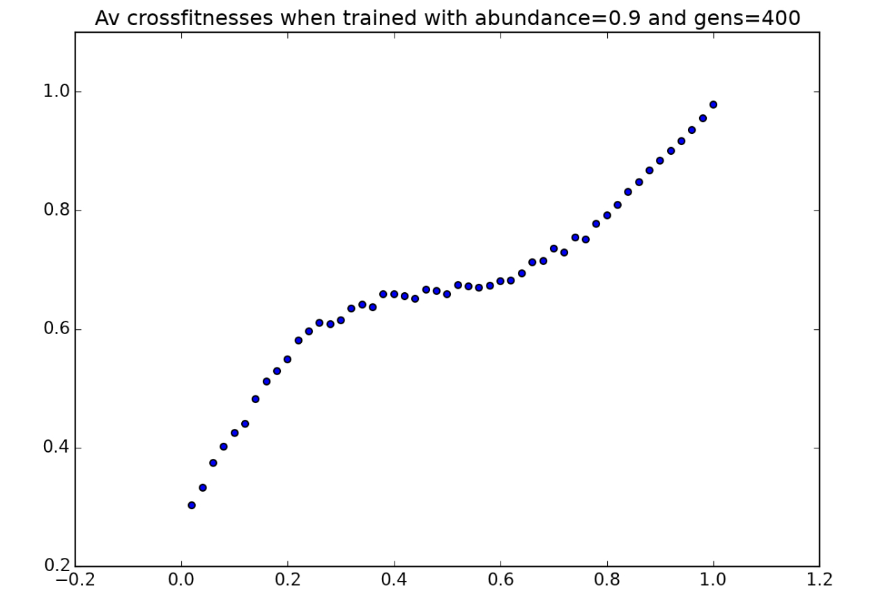
and here are three more sample players accustomed to high-abundance environments:
In all three of these animations, the players can be seen using the same strategy: when they can’t see any tokens, they move in one direction rather than in a random direction. Why might this strategy be more favorable in environments with higher token abundance?
The answer to this question becomes obvious when we watch these same three players play in environments with $a=0.3$:
That’s pretty pitiful - most of them get stuck running in circles very quickly. It makes sense that this strategy might not be so bad when there are lots of tokens, since the player is more likely to bump into another random clump of tokens by moving in a straight line. However, when tokens are sparse, entire rows or columns could be entirely devoid of tokens, and the player could get stuck cycling through those columns forever without checking for tokens elsewhere.
Here’s a summary of all of the important points we’ve noticed in this section:
At this point, we could have a look at how tweaking other environmental factors, like the size of the gameboard and the number of turns players are allowed, affect the strategies that develop. However, since this blog post has already stretched out much longer than I’d expected, I’ll limit it to exploring the effects of different token-abundance values.
There’s another type of experiment I’d like to try as well, though I think I’ll save it for another post. It would be interesting to let a population evolve in one environment for $100$ to $200$ generations before transplanting it into a different environment and letting it continue to evolve there. Lots of its old strategies would probably be overwritten, but then again, some “vestigial” strategies might remain, possibly allowing the player to be more versatile and perform well across a broader range of different environments.