Polyhedra in STL and the Conway Operators

Since last November, I’ve been working as a research assistant at Leah Buechley’s Hand and Machine computational design lab at UNM. The MO of computational design is to use code to generate two-dimensional designs or three-dimensional structures that are aesthetically appealing or have unique physical properties. There’s a heavy emphasis on the intersection between the abstract, algorithmic side of computer science and the concrete mechanical side: algorithmically designed patterns or structures are manifested in a physical substrate such as textiles, ceramics, or plastic using textile machines or 3D printers. For the past few months I’ve been busy experimenting with the Prusa i3 MK3 3D printer for my job (which is partly why I haven’t written a post in so long), and the purpose of this post is to document some of the interesting problems that I’ve enjoyed solving so far. In particular, I’ve been working on writing a Python framework for constructing, manipulating, and transforming 3D polyhedra, which has posed all sorts of cool algorithmic and geometrical puzzles.

STL file format

One of the first things I learned about was STL, a file format used often in computer-aided design to generate 3D-printable models of solids. A compelling perk of this format is that it can be written in ASCII, and is extremely human-readable. Here’s an example of an ASCII STL file describing a regular tetrahedron of unit side length:

solid unit-regular-tetrahedron    
facet normal 0.0 0.0 -1.0     
outer loop  
vertex 0.5773502691896258 0.0 0.0   
vertex -0.2886751345948128 -0.5000000000000001 0.0   
vertex -0.2886751345948132 0.4999999999999999 0.0   
endloop  
endfacet  
facet normal 0.4714045207910318 -0.8164965809277259 0.3333333333333335   
outer loop  
vertex -0.2886751345948128 -0.5000000000000001 0.0   
vertex 0.5773502691896258 0.0 0.0   
vertex -1.8503717077085938e-17 0.0 0.8164965809277259   
endloop  
endfacet  
facet normal -0.9428090415820632 -3.663549070262141e-16 0.33333333333333354   
outer loop  
vertex -0.2886751345948132 0.4999999999999999 0.0   
vertex -0.2886751345948128 -0.5000000000000001 0.0   
vertex -1.8503717077085938e-17 0.0 0.8164965809277259   
endloop  
endfacet  
facet normal 0.4714045207910314 0.8164965809277261 0.33333333333333326   
outer loop  
vertex 0.5773502691896258 0.0 0.0   
vertex -0.2886751345948132 0.4999999999999999 0.0   
vertex -1.8503717077085938e-17 0.0 0.8164965809277259   
endloop  
endfacet  
endsolid unit-regular-tetrahedron  

Here’s what each of these keywords does:
- solid begins the description of a solid with a specified name, and endsolid marks the end of the description
- facet marks the beginning of the description of a facet, and endfacet marks the end. A facet of an STL solid is basically the same as a face, but STL facets have a few quirks that I’ll mention momentarily.
- normal declares the normal vector to a facet.
- outer loop declares the beginning of a list of vertices, and endloop marks the end of the list.
- vertex declares a vertex with given coordinates as a vertex of the current facet.

And finally, here’s what the solid described by this STL file looks like:

This doesn’t work exactly how we would expect it to work at first glance, though. For one thing, all facets must be triangles - no polygons with more than 3 sides are allowed. This means that if you want to generate an STL file for, say, a cube, rather than representing the cube in terms of its 6 faces and their vertices, you would have to dissect each square face into 2 triangles and represent the cube using these 12 triangles. Another curveball is the fact that each facet is only "visible" from one side, which is determined by the normal vector. Although the above STL model displays a tetrahedron when the vantage point lies outside of the tetrahedron, nothing is visible from a vantage point inside of the solid, since only the "outside" side of each facet is visible. For example, here’s an STL file containing only one triangular facet that is visible from only one side (you might have to drag it around a little bit before you see anything):

If you know your trigonometry, manually writing out STL files for more complex solids is easy but quickly becomes tedious. The process of breaking up more complex polygons into triangles and explicitly writing out each triangle’s vertices and normal vector is just begging to be automated. It’s a pretty simple exercise in Python file I/O to write an STL file given a list of vertices and normal vectors for various triangles.

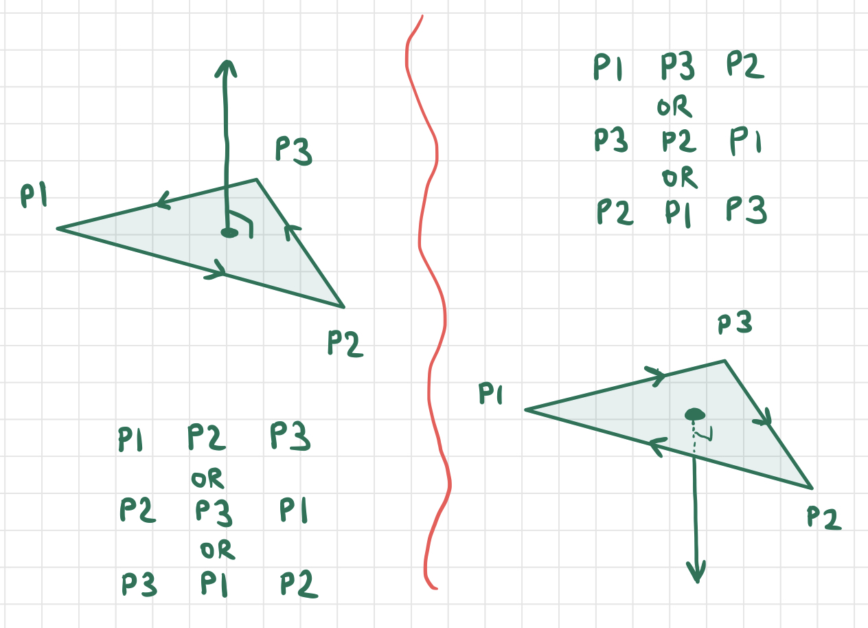
A less trivial exercise, however, is to write Python code that generates STL triangles given only a list of their points with no normal vector. At first this seems like an ambiguous way to identify a facet, since any triangle defined by three vertices corresponds to two possible facets - one for each flat "side" of the triangle that can be viewed. However, we can disambiguate between the two possible facets by paying attention to the order in which the points of the triangle are listed. In particular, we say that the sequence of points $P_1,P_2,P_3$ pick out the facet of the triangle from which these three points appear in clockwise order around its boundary. Note that the sequences of points $P_2,P_3,P_1$ and $P_3,P_1,P_2$ pick out the same facet as $P_1,P_2,P_3$. However, the sequence $P_1,P_3,P_2$ picks out the opposite facet of the triangle.

Let’s suppose the three vertices of a triangle are given in the order $\vec x, \vec y, \vec z$ and use this to calculate the normal vector of the corresponding facet. The vectors $\vec x - \vec y$ and $\vec z - \vec y$ correspond to two sides of the triangle pointing away from the vertex $\vec y$, and by applying the right-hand rule of vector cross-products, we can see that the normal points in the direction of

$$(\vec x - \vec y)\times (\vec z - \vec y)$$

Knowing this formula, it becomes pretty easy to write Python code computing the facet normal given the three clockwise vertices defining the facet. If we want, we can convert this to a unit normal vector by dividing it by its own magnitude $||(\vec x - \vec y)\times (\vec z - \vec y)||$.

Redundancy in storing polyhedra

Now that we’ve talked about how STL files and oriented facets work, it’s simple to see how to convert a given solid into an STL file. If we have a list of faces and a list of vertices (in counterclockwise order) for each face, all we need to do is dissect each face into triangles and add these triangles to the STL file. But now the question is - how can we explicitly calculate the vertex coordinates (and which vertices are on each face) of interesting solids that we might want to render using STL, for instance the Platonic solids or the Archimedean solids (or maybe even all of the Johnson solids)? Or, given a simple solid, how can we transform its vertices and faces to produce a more complex solid that can be rendered as an STL file?

Part of what I’ve been working on for my job at Hand and Machine is developing a Python framework for manipulating polyhedra and converting them to STL files. One of the most salient lessons I’ve learned is the power of redundanct data structures to make more efficient code. For example, in my code, a Solid object is defined mainly by a list of vertices with ID numbers and a list of faces that refer to the vertices by their IDs. A Solid can be built up from nothing by progressively adding vertices and faces that refer to those vertices. Now suppose we want to write a method for the Solid class that returns all of the "neighbors" of a given vertex, that is, all of the vertices that are adjacent to a given vertex along an edge. If a Solid is structured as described above, the following pseudocode describes an algorithm for generating a list of all of the "neighbors" of a given vertex:

given a vertex v  
create empty list neighbors   
for each face f in solid:  
    if v in f:  
        get the vertices n1, n2 next to v  
        add n1, n2 to v  
return neighbors  

This algorithm works, but it wastes a lot of time. The complexity is $\mathcal{O}(f)$ where $f$ is the number of faces in the Solid, but most of the faces being checked probably don’t even contain the vertex v. On the other hand, if we change what information is calculated and stored in the Solid object as it is being built, we can implement this functionality in $\mathcal{O}(1)$. Suppose that, in addition to a list of vertices and faces, each Solid object also contains a list of "neighbors" of each vertex, and that these lists are updated each time a new vertex or face is added to the Solid. Each update costs $\mathcal{O}(1)$ time, leaving the time complexity of building the Solid unchanged - but now getting the neighbors of a vertex is as easy as returning a pre-built list, which is trivially $\mathcal{O}(1)$. Even though these lists of vertex neighbors contribute no new information about the Solid that wasn’t already present in its vertex and face lists (i.e. they are redundant), they drastically speed up the process of finding vertex neighbors!

For similar reasons, I’ve incorporated redundant data structures for each of the following pieces of information as well:

• The total number of vertices in the Solid
• Lists of all faces containing a given vertex
• Lists of all faces containing a given pair of vertices
• The number of vertices in each face
• The position of a given vertex on a given face, given the vertex’s ID

The last two pieces of information aren’t stored in Solid, but rather in each Face object.

Conway polyhedron operators

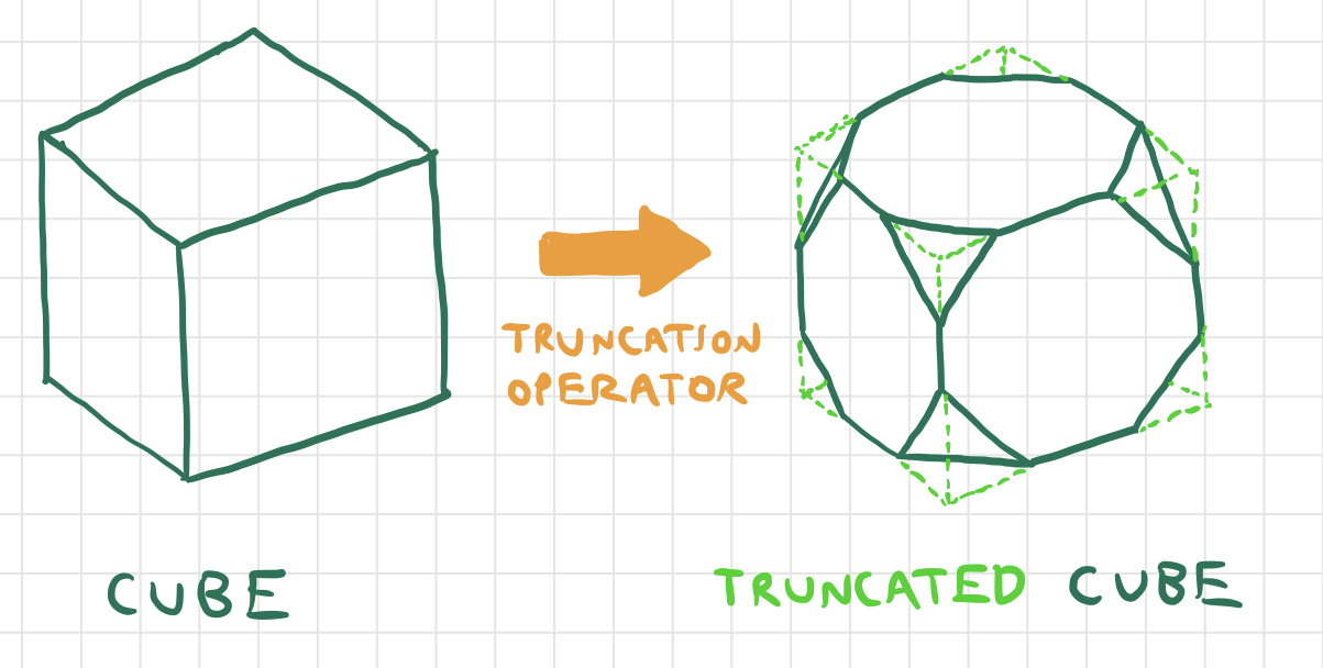
Generating all of the Platonic solids was an interesting challenge, and I wrote a few "helper" functions to abstract some commonly-occurring geometric constructions, but most interesting challenges came when I started working on the Archimedean solids. Many Archimedean solids can be obtained by applying an (intuitively) simple operation to a Platonic solid. For instance, several Archimedean solids are just truncated versions of their Platonic counterparts - that is, Platonic solids with the corners chopped off. For example, truncating the corners of the (Platonic) cube yields the (Archimedean) truncated cube:

By writing a function to chop the corners off of any Solid, I could generate the following Archimedean solids in one swoop, rather than constructing their faces and vertices manually:

• truncated tetrahedron
• cuboctahedron
• truncated cube
• truncated octahedron
• icosidodecahedron
• truncated dodecahedron
• truncated icosahedron

It turns out that the truncation operator is just one of many polyhedron operations called the Conway polyhedron operations that can be used to manipulate existing polyhedra. Another one is called the "expand" operaton, which pushes all of the polyhedron’s faces away from its center and then "fills in the gaps" with more faces. The rhombicuboctahedron and rhombicosidodecahedron can be obtained by applying the "expand" operator to the cube and the dodecahedron respectively. The "snub" operator is similar to the "expand" operator, but it involves twisting the faces in addition to translating them outward, and it can be used to generate the snub cube and snub dodecahedron. In addition to their utility for generating the Archimedean solids from the Platonic solids, the Conway operators are just fun to play with, and can be used to create all sorts of intricate and symmetrical solids from simpler ones.

One more important note before we get into the weeds - the Conway polyhedron operations are actually topological, not geometrical. In other words, they tell us how to change the ways in which the faces/edges/vertices of a solid are connected to each other, but not where the vertices of the new solid should be situated in space. They operate on the graph of a solid, not its manifestation in 3-space. For example, the "kis" operation tells us to create a new vertex for each face, and connect the vertices of each face to the new vertex corresponding to this face. But there are many solids in 3-space that fit this description, because the "new points" can be placed anywhere. Here two different solids that could result from applying the "kis" operation to a cube:

Similarly, with the truncation operator described earlier, there is a choice for each vertex about "how deep" and at what angle each vertex is "chopped off". This means that most of the Conway operations I’ve implemented take additional arguments that parametrize the result of the operation in some way (by allowing the user to specify, for example, the depth of truncation or the "spikiness" of a solid produced by truncation).

The kis operator

To get warmed up, here’s pseudocode describing my implementation of the "kis" operator, which was by far the easiest:

given a solid s and a height h  
create a new empty solid s’  
for each face f in s:  
    let c be the centroid of f  
    let n be the unit normal vector of f  
    p = c + n * h  
    for each vertex v in f:  
        let v’ be the next vertex of f counterclockwise from v  
        let f’ be the face defined by v, v’, p  
        add f’ to s’  
return s’  

This algorithm is $\mathcal{O}(n)$ where $n$ is the number of vertices of the solid. For large values of h, this will generate increasingly "spiky" solids, whereas for negative h, it will generate a "caved in" version of the original (the first example with the cube corresponds to positive h, and the second to negative h). When h equals zero, we’ll get a solid with four times as many faces that looks identical to the original because many of the faces will be coplanar to each other. This algorithm is pretty simple, but there’s one important thing worth pointing out - where I defined f’ as the face defined by the vertices v’, v, p, note that this order matters since our "faces" are actually facets whose orientations are defined by the order in which their vertices are listed. Recall that for the "outside sides" of our solid to be visible, their vertices must be listed in counterclockwise order as viewed from the outside. Take a moment to visualize a free-floating face in space, a point p elevated some height h above this face, and two vertices v, v’ in counterclockwise order on the perimeter of this face, and convince yourself that the facet v, v’, p appear in counterclockwise order as viewed from outside the solid, whereas v’, v, p do not appear counterclockwise.

The truncation operator

Next, here’s my pseudocode algorithm for truncation. It’s greatly simplified, and several of the steps are trickier than they seem, which I’ll comment on afterwards.

given a solid s and a proportion p  
copy s into the new solid s’  
for each vertex v in s:  
    let evs be the list of vectors pointing from each of v’s neighbors towards v  
    let uevs be the list of unit vectors corresponding to the vectors in evs  
    let cut be the normalized average of all unit vectors in uevs  
    let projs be the list of the projections of each vector in evs onto cut  
    let minproj be the length of the shortest vector in projs  
    d = p * minproj  
    replace s’ by the solid formed by truncating vertex v from s’ with a cut depth of d  

Intuitively, this algorithm calculates the direction in which each truncation cut will be made (the average direction of the edges connected to a given vertex), figures out how deep each cut can be made without colliding with any adjacent vertices, and makes cut that are a proportion p of this maximum depth for each vertex. This part is easy and algorithmically uninteresting - it’s just a bunch of vector algebra. The hard part is in the details of the last line. How do we find the solid formed by truncating a single vertex of another solid?

My first attempt was to write a more general function which, given a solid and a plane, would find the solids formed by slicing that solid across the given plane. Then I used this function to make a plane slice near each of the solid’s vertices, "chopping off" each of its vertices. My plane-slice algorithm, however, was horribly inefficient, and only worked reliably for convex solids. This is because a plane slice at one vertex of a concave solid may also intersect the solid somewhere else, "accidentally" chopping off more than the tip of one vertex.

Here’s one of the earlier algorithms that I used - it works for convex as well as concave solids, but contains an inefficient step:

given a solid s, a vertex v on s, and a depth d  
create an empty solid s’  
let uevs be the list of unit vectors pointing from each of v’s neighbors towards v  
let cut be the normalized average of all unit vectors in uevs  
cut = -cut  
p = v + depth * cut  
let pl be the plane defined by the point p and the normal vector cut  
let newvs be the list of points at which pl intersects the edges connected to v  
sort the points in newvs in clockwise order about the vector cut  
add the face defined by the points in newvs to s’  
for each face f in s containing v:  
    let p1, p2 be the points on f adjacent to v, in counterclockwise order  
    let q1 be the point where pl intersects the edge from p1 to v (already calculated in newvs)  
    let q2 be the point where pl intersects the edge from v to p2 (already calculated in newvs)  
    let pts be a copy of the list of vertices in f  
    in pts, replace v with the points q1, q2 in that order  
    add the face defined by the points in pts to s’  
add all faces of s not containing the vertex v to s’  

The inefficient step here is sort the points in newvs in clockwise order about the vector cut. Because it involves sorting a set of $n$ points where $n$ is the number of neighbors of v, it will be $\mathcal{O}(n\log n)$, whereas the rest of the algorithm is $\mathcal{O}(n)$. If we could find a way to get these points in clockwise order without having to sort them, it would lower the complexity of the entire function! (In practice, a complexity of $\mathcal{O}(n\log n)$ isn't actually that bad compared to $\mathcal{O}(n)$ - probably the most computationally costly step is computing all of the angles between the vectors, not sorting them, even though the latter asymptotically dominates the former for very large polyhedra. Thanks to my friend CJ for pointing this out!)

It turns out that it’s possible to build the list newvs in such a way that the points appear in the correct order without performing the expensive operation of sorting them. This can be accomplished using the following steps:

let newvs be an empty list  
let avs be an empty list  
let av be any vertex adjacent to v  
repeat a number of times equal to the number of neighbors of v:  
    add av to avs  
    get the face containing the edge from v to av, in that order  
    let av’ be the vertex before v (counterclockwise) on that face  
    av = av’  
for each vertex v’ in avs:  
    let newv be the point where the plane pl intersects the plane joining v to v’  
    add newv to newvs  

The list ‘avs’ will contain the neighbor vertices of v in such a way that their respective edges with v wrap counterclockwise about the "corner" at v, or clockwise about cut, which points towards the interior of the solid. Why does the construction turn out this way? It leverages information about clockwise/counterclockwise orientation already stored within the solid, namely the fact that the vertices of each face are listed in counterclockwise order as viewed from the outside. This means that if we draw a star-shaped path through v and its neighbors in such a way that it always moves in the direction opposite the orientation of the edges of the faces, it will wind about v in a counterclockwise orientation. Here’s a diagram to help visualize what’s going on:

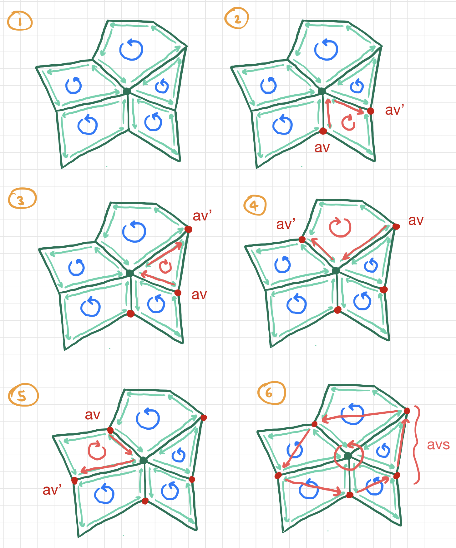
This algorithm is $\mathcal{O}(n)$ in the number of neighbors $n$ of the vertex v. Note that the steps like get the face containing the edge... can be completed in $\mathcal{O}(1)$ time because of some of the redundant data structures built into the solid, described at the end of the previous section. This brings the complexity of the whole truncation algorithm down to $\mathcal{O}(n^2)$.

The dual operator, and face smoothing

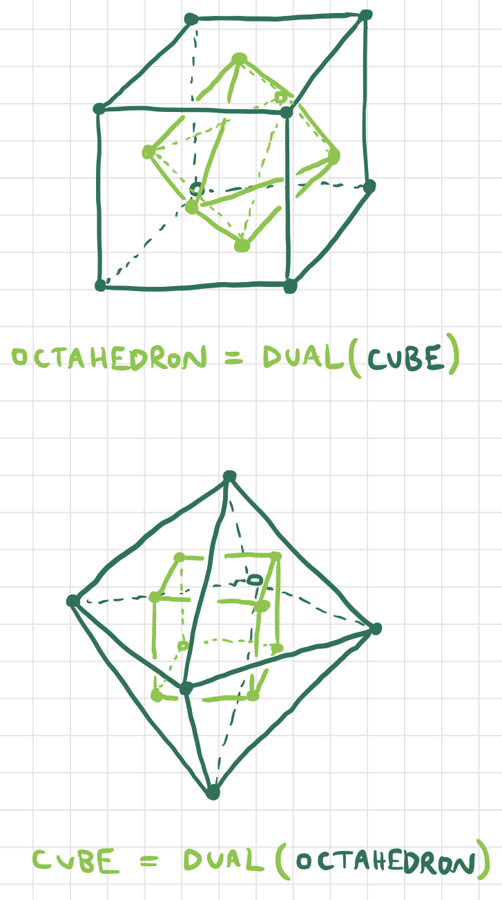
There’s one more operator I’d like to discuss, which is the dual operator. The (topological) dual of a solid is formed by replacing each of the faces with vertices and each of the vertices with faces, in such a way that two vertices are connected by an edge if and only if their corresponding faces shared an edge, and two faces share an edge if and only if their corresponding vertices were connected by an edge. There are lots of nice relationships between the Platonic and Archimedean solids in terms of the dual operator: for example, the cube and the regular octahedron are duals of each other, as are the regular dodecahedron and the regular icosahedron.

The most obvious way to find the dual of a solid is to compute the centroid of each face and draw edges connecting each pair of centroids corresponding to faces that border each other. We can write this algorithm in pseudocode as follows:

given a solid s  
create a new empty solid s’  
for each face f in s:  
    let c be the centroid of f  
    add c as a vertex of s’  
for each edge e in s:  
    let f1, f2 be the faces on either side of e  
    add an edge to s’ joining the centroids of f1 and f2  

This algorithm is $\mathcal{O}(n)$ in the number of faces $n$ on the original solid. So what’s the big deal? This algorithm seems simple enough, right?

Well, the resulting collection of vertices and edges will topologically be the dual of the original solid, but it’s not even guaranteed to be a well-defined 3D polyhedron. This is because this process does not guarantee that a collection of vertices that are connected by edges to form a face are actually coplanar. In other words, for some input solids s, the above process results in s’ having "degenerate faces" whose vertices don’t actually lie in the same plane! These "degenerate faces" can be rendered in STL by splitting them up into multiple nondegenerate triangular faces, but although this makes it possible to visualize the resulting solid in 3D, it alters its topology so that it is no longer the topological dual of the original solid. Here’s a picture of one of the Archimedean solids and its dual with degenerate faces:

If you could stick your fingers into that picture and shift the solid’s vertices and faces around manually, it almost feels like you could "shimmy" them around a little bit to make all of the triangles line up and the degenerate faces become regular faces. But this is not a precise mathematical algorithm. We need to find a way to turn degenerate faces whose vertices are almost coplanar into faces whose vertices are, in fact, coplanar.

The easiest way to make sure a bunch of vertices lie in the same plane is to pick a plane and project them onto it. Consider one face $F$ with points $P_1, P_2,..., P_n$ that are not coplanar. For a face that is nondegenerate, the plane in which all of its points lie is precisely that plane which passes through that face’s centroid and is normal to the normal vector to that face. Now, $F$ doesn’t exactly have a centroid since its vertices are noncoplanar - but the centroid of an ordinary face can be found by averaging the coordinates of its vertices, so we can generalize by saying that the "centroid" of $F$ is the point found by averaging the coordinates of $P_1,P_2,...,P_n$. Call this "centroid" $C^\star$. Similarly, $F$ doesn’t exactly have a normal vector - but the triangle $\triangle P_1P_2P_3$ has a normal vector, and so does the triangle $\triangle P_2P_3P_4$, and so on, so we might call the vector formed by averaging the normal vectors of each of these triangles the "normal vector" of $F$. Let’s denote this "degenerate normal vector" $\vec{n}^\star$. Now we can project each point $P_i$ onto the plane defined by $C^\star$ and $\vec{n}^\star$ to obtain a set of points that are both coplanar and reasonably close to the originals. The projection of the point $P_i$ onto this plane can be calculated as

$$C^\star + \text{proj}_{\vec{n}^\star}(\overrightarrow{C^\star P_i})$$

So, now we’ve come up with a way to "planarize" the vertices of one degenerate face. But we have another problem: all of the faces of a solid are connected to each other. If $F_1$ and $F_2$ share some vertices, and we planarize $F_1$ and then planarize $F_2$, the vertices of $F_1$ might not be coplanar anymore, since we will have shifted a few of them while planarizing $F_2$. Is there a way to planarize all faces of our solid at once, so that we don’t "mess up" previously planarized faces?

Suppose $P_i$ is some point on our solid, and $F_a$ and $F_b$ are two degenerate faces containing it. Define $P_{ia}’$ to be the image of the point $P_i$ when $F_a$ is planarized, and $P_{ib}’$ be the image of $P_i$ when $F_b$ is planarized. The fact that $P_{ia}’$ and $P_{ib}’$ are not necessarily equal is why we’re in trouble - the planarizations of two degenerate faces might disagree with each other. So why don’t we compromise by averaging these images with each other? More precisely, if the point $P_i$ is on the faces $F_{a_1}, F_{a_2}, ... F_{a_k}$, then the "compromise point" formed by averaging its images under the planarization of each face is given by

$$\bar{P_{i}’} = \frac{1}{k}\sum_{n=1}^k P_{ia_k}’$$

(Where the points are summed componentwise.) Now, if we replace each point $P_{i}$ by the point $\bar{P_{i}’}$, we still aren’t guaranteed a solid with nondegenerate faces, but we should get something closer to a nondegenerate solid - the degenerate faces should be "smoothed out" to some extent as each of the vertices of each face are shifted towards a common plane. If we apply this process many times, hopefully the degenerate faces will become smooth enough that their irregularities are no longer noticeable, and they become approximately equal to nondegenerate faces. Remember the degenerate dual of the Archimedean solid we saw earlier? Here’s what happens when we repeatedly apply this smoothing algorithm:

After only three iterations, it’s hard to tell the difference, and after even more iterations, the vertices of each face are so close to being planar that we’ve essentially solved the problem. The best part is that this algorithm isn’t just restricted to degenerate polyhedra obtained by applying the dual operator. Given any collection of points and edges haphazardly scattered in 3D space, we can apply this algorithm to smooth it out into a nice nondegenerate polyhedron. Of course, this won’t work for configurations of points and edges that aren’t topologically polyhedral (e.g. if their faces aren’t closed or something nasty like that), or if the points of each face aren’t even close to being planar.

Conclusion

There are several other challenges that I didn’t have time to write about in this post, such as

• the specific geometrical tools/functions that I wrote to help construct the original Platonic/Archimedean solids
• dealing with floating-point errors when storing vertex coordinates
• algorithmically computing the convex hull of a set of points
• a few other Conway operators that I implemented, such as the "expand" and "snub" operators

Also, I’ve been 3D printing many of the polyhedra I’ve designed while working on this framework, and 3D printing has introduced some interesting puzzles of its own. More recently I’m experimenting with directly editing the GCODE of 3D prints, or the files that dictate the exact movements that the machine must take to create a particular structure. Perhaps that will be the topic of a future blog post.

Please enjoy the following polyhedra in parting, which were constructed by repeatedly applying different Conway operators to Platonic and Archimedean solids: