
In this post, I will describe a mathematical process that can be used to compress images (and probably also other types of large files). Fully understanding this post will require a bit of background knowledge from linear algebra. However, I’ve tried to explain all portions of this post in layman’s terms as well, so that it is comprehensible to readers without a technical background. It might get a bit dense, but don’t give up even if the mathematical notation or terminology is foreign - I will try to simplify the complicated bits and restate them in plain English.
Digital files like audio, images, and video are notoriously bulky, occupying an unwieldy amount of storage space and taking an inconveniently long time to send to other devices. This is because, unlike text files, they contain fine detail. Suppose I send you a text file that is $400$ characters long and there are about $30$ different characters that I could type (including letters, spaces, and punctuation). Then using the measurement of information content that is widely accepted in information theory, the information content of my message would be somewhere around
bits of information. However, suppose that instead I want to send you an image that is $400\times 400$ pixels large. Each pixel in the image would have to store a color value, not a letter of punctuation mark, and there are certainly more than $30$ different colors that are distinguishable to the naked eye. This means that the information content of the image would be at least
That’s more than $300$ times our estimate for the information content of the text file! Now consider a video, in which each frame is a $400\times 400$ pixel image, and perhaps there are $100$ different frames (even $100$ frames would only make for a very short video, or a very choppy one). Then the estimated information content, excluding whatever information is included in the audio, would be at least
Yikes, that’s greater than the number of atoms in the universe! These are all probably overestimates, since most text, image, and video files usually have some kind of redundancies or predictable components that reduce their information content, but these approximations at least demonstrate the gargantuan order of magnitude of the information content of a video file.
So, of course, when sending images and audio and video files, we have to make use of compression techniques that squeeze large files into smaller ones. Sometimes it’s possible to compress a file so that it occupies less space and can be recreated in its exact form, but this isn’t always possible. Sometimes we have to sacrifice the quality of a photo or video in order to reduce its size, which means that some of the original information stored in the file is discarded or lost when it is compressed.
For instance, suppose I wanted to send you a message by telegram, but that I was being charged by the letter and was too stingy to waste money on telegram messages. Then I might save money by sending you an altered version of my message with all of the vowels removed:
“Mt m n th twn sqr t mdnght.”
It’s tricky and inconvenient to read, but you could probably deduce what I’m trying to convey:
“Meet me in the town square at midnight.”
The same idea applies for images and videos.
However, it’s worth noting that in some cases, information can be trimmed from an audio, image, or video file without inconveniencing the viewer at all. The field of perceptual coding takes advantage of human sensory biology to optimize information storage and eliminate extraneous information. Humans can’t distinguish between certain colors, hear certain tones, or consciously register visual changes that occur too quickly. Thus, any media that we consume can be entirely stripped of this imperceptible information and the viewer won’t even be able to notice the difference!
We won’t be getting into anything so advanced in this blog post. I don’t even know if SVD Decomposition is currently used to compress images, and there are probably far more advanced and efficient methods for doing so. However, it nonetheless serves as an interesting and illustrative example.
Let’s start digging in to the mathematics behind SVD Decomposition. Suppose you have an image file that you want to store (for simplicity’s sake, we’ll consider only black-and-white images). The color of each pixel (in black-and-white, these will all be different shades of gray) can be represented as a decimal value encoding that pixel’s brightness, and these numerical values can be stored in a table or two-dimensional array called a matrix, like this:
For example, if the number $0$ represents a completely black square and the number $100$ represents a completely white square, this $3\times 3$ pixel image
could be stored in the following matrix:
There’s a special type of matrix called a rank 1 matrix that is very simple and easy to express compared to other matrices. If you’re familiar with linear algebra, you should know what “rank 1” means, but if not, here’s a quick explanation. A matrix has rank 1 if all of its columns are multiples of a single column. For example, consider the matrix
In this matrix, all of the columns are multiples of this column vector:
More specifically, the first column of $A$ is $5\vec{c}$, the second column of $A$ is $2\vec{c}$, the third is $3\vec{c}$, the fourth is $0\vec{c}$, and the fifth is $-2\vec{c}$. To use a bit of linear algebra terminology, we can say that the matrix $A$ is the outer product of the column vector $\vec{c}$ with the row vector $\vec{r} = \langle 5,2,3,0,-2\rangle$:
Notice that if I told you the entries of $\vec{c}$ and $\vec{r}$, you could completely reconstruct $A$ without me explicitly sending you all of the values stored in $A$. But $\vec{c}$ and $\vec{r}$ together store only $3+5=8$ numerical values, while $A$ stores a total of $3\cdot 5=15$ numerical values. So by encoding $A$ as the outer product of $\vec{c}$ and $\vec{r}$, we can get away with using only $8$ numbers to store $A$, rather than $15$.
Suppose that $A$ was a much larger matrix, say $300\times 500$, instead of just a wimpy little $3\times 5$ matrix (after all, we don’t often deal with image files that are only $3\times 5$ pixels). Storing $A$ in its raw form would require us to store $300\cdot 500=150,000$ different numerical values. However, if $A$ has rank 1, then it can be written as the outer product of a $300$ -element vector $\vec{c}$ with a $500$ -element vector $\vec{r}$: If this is the case, then we don’t have to store all of the values in $A$, but only the values in $\vec{c}$ and $\vec{r}$, which is only $300+500=800$ numerical values. Given that storing $A$ unmodified would require remembering $150,000$ different numbers, a compression technique bringing this figure down to only $800$ seems pretty impressive!
The problem is that this only works for matrices with rank 1. There are plenty of matrices that don’t have rank 1, and in fact very few image files that we would ever want to store or transmit have this property. However, a theorem from linear algebra states that any $m\times n$ matrix can be written as a sum of at most $\min(m,n)$ different rank 1 matrices. More specifically, for any $m\times n$ matrix $A$, there exist constants $\sigma_i$ and vectors $\vec{u_i},\vec{v_i}$ such that
where $p=\min(m,n)$. This is Singular Value Decomposition! Similarly, the constants $\sigma_i$ are called the singular values of the matrix $A$.
As we noticed earlier, if $\vec{u_i}$ is an $m\times 1$ vector and $\vec{v_i}$ is an $1\times n$ vector, the outer product $\vec{u_i}\otimes \vec{v_i}$ is an $m\times n$ matrix with $mn$ elements, but all of the information it contains can be stored simply by storing the $m+n$ values contained in $\vec{u_i}$ and $\vec{v_i}$. Similarly, the weighted outer product $\sigma_i\vec{u_i}\otimes \vec{v_i}$ can be completely stored using only $m+n+1$ values (since we must also hold on to the value $\sigma_i$). Thus, if $A$ can be decomposed into at most $\min(m,n)$ terms of this form, then all of the information in $A$ can be stored using only $(m+n+1)\min(m,n)$ values. Unfortunately, this isn’t very helpful, because, as it turns out, the following is true for all $m,n\in\mathbb N$: so storing $A$ by storing the values in each of its components would actually require more storage space, not less (unless, by pure chance, the matrix $A$ can somehow be broken down into fewer than $\min(m,n)$ rank 1 matrices).
However, suppose, for instance, that we have an image stored in a $5\times 5$ matrix $A$ that can be broken down as follows: Storing $A$ in its raw form would require us to store a total of $25$ values, while storing the singular values $\sigma_i$ and the vectors $\vec{u_i},\vec{v_i}$ would require us to store $55$ values, making it extremely inefficient. However, notice that the last three singular values $0.01,0.007,0.001$ are very small compared to the first two $5,3$, meaning that the last three terms $E_3,E_4,E_5$ don’t actually change the value of $A$ very much. So if we wanted to approximate $A$, we might write that Storing the singular values $\sigma_1,\sigma_2$ and the values in the vectors $\vec{u_1},\vec{v_1},\vec{u_2},\vec{v_2}$ would only require us to store a total of $22$ values, compared to the $25$ values required to store $A$ as it is. Thus, if we’re willing to sacrifice the accuracy of $A$ a little bit, we can store it using less space. If $A$ is storing an image, this “compressed” form of $A$, given by $E_1+E_2$, might be a bit fuzzier, grainier, or less detailed than $A$ in its full glory, but it would also occupy less space. In a moment we’ll perform SVD decomposition on an actual image and see what happens when we truncate its decomposition.
The above section was a bit heavy on mathematical notation and terminology, so here’s a summary. If we have an image that we want to store, we can break it down into a “sum” of many simpler images that are easier to store. Then, we can figure out which of these simpler images are most important and discard the ones that are least important or encode the finest detail. This allows us to “approximate” the image by sacrificing some detail or image quality in order to store it using less space.
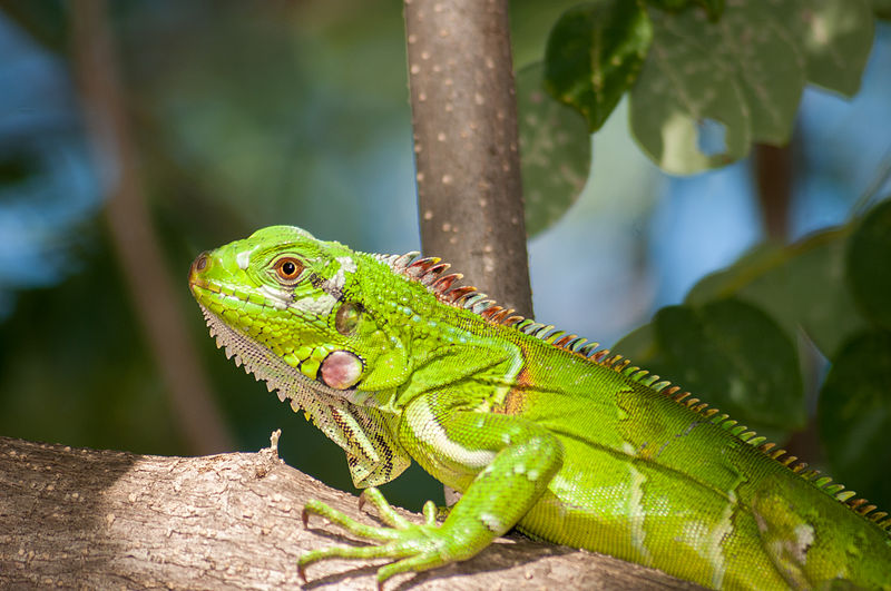
Now let’s try this out with an actual image. Check out this $531\times 800$ pixel image of a gorgeous iguana:
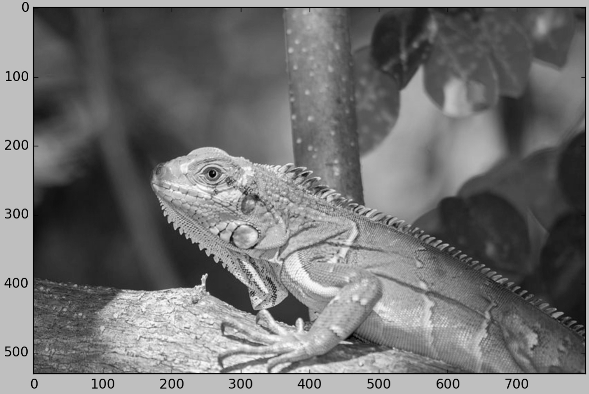
To make things simpler, we’ll only be dealing with a black-and-white version of this image. Here’s what it looks like when stored as a matrix and plotted using Python:
Decomposing the image using a special function in Python shows that its SVD expansion (as a weighted sum of rank 1 matrices) does in fact have the $531$ terms. We can represent the decomposition as follows:
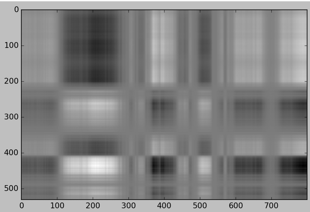
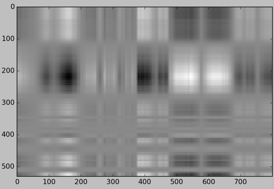
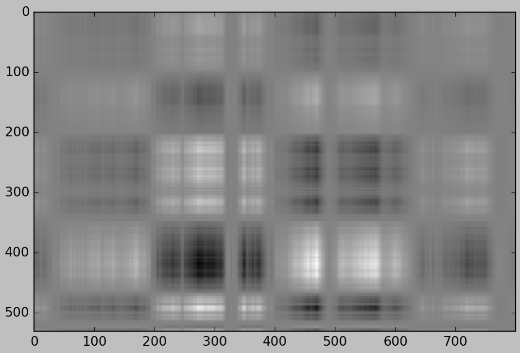
Let’s have a look at a few individual terms $E_i$ of this expansion. Each term is a matrix that corresponds to an image, so we can isolate and display the image corresponding to any of the $E_i$. Here are the images corresponding to $E_1$ through $E_5$:
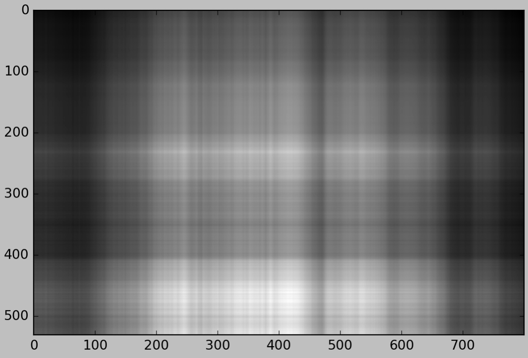
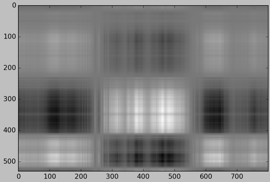
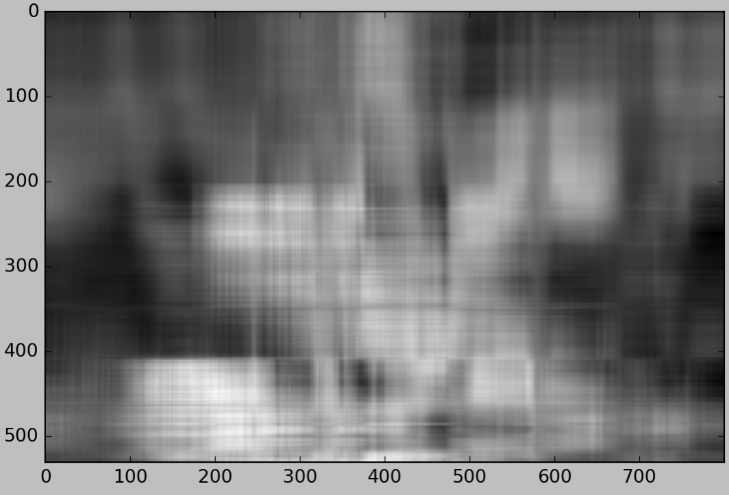
They don’t look like much of anything, right? When we add them together, however, they begin to bear a hazy resemblance to the original image. Here is the image corresponding to the sum of the first $5$ terms $E_1+E_2+E_3+E_4+E_5$:
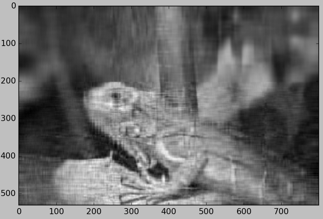
It still doesn’t look like an iguana, but it begins to come together if we add a few more terms. Here’s the image corresponding to the sum of the first $10$ terms $E_1+...+E_{10}$:

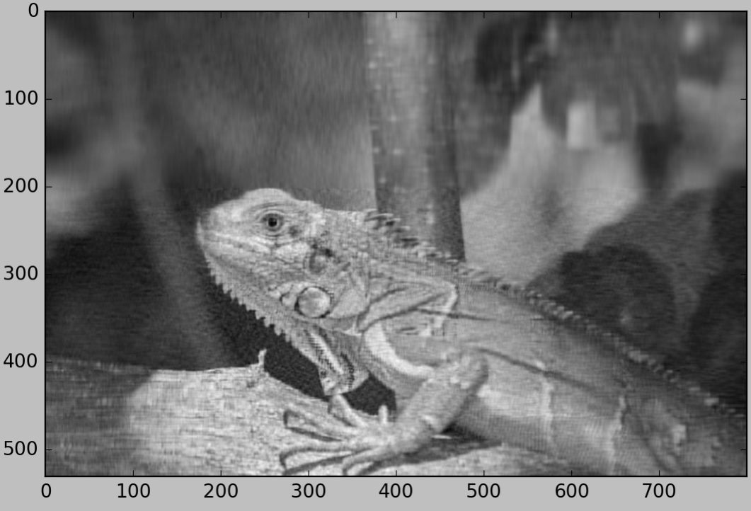
The quality is still very poor, but it is beginning to look like an iguana (or at least some sort of creature) sitting on a surface. Its black eye and its long, spindly fingers are now clearly visible. Tacking another $10$ terms onto the approximation gives us the following image:
This is now clearly an iguana. Let’s jump ahead to the 50-term approximation $E_1+...+E_{50}$:
and here is a 100-term approximation:
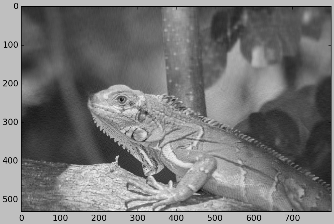
This image is pretty high-quality. It’s visibly grainy in the background area surrounding the iguana, but the texture of the iguana’s skin and the log make it difficult to see any flaws in those portions of the image. Keep in mind that this approximation only uses $100$ terms of the $531$ total terms in the image’s SVD expansion. This image is very close to the original, yet it uses fewer than $1/5$ of the terms! Recall that storing one of the $m\times n$ rank 1 matrices $E_i$ requires the storage of $m+n+1$ numerical values. This means that storing the 100-term approximation of this $531\times 800$ images requires us to store $(531+800+1)\cdot 100=133,200$ values, while storing the iguana image in its full glory would require us to store $531\cdot 800=424,800$ values. Thus, our decent 100-term approximation could be stored using a little less than $1/3$ of the space required for the original.
Not impressed? Check out this 200-term approximation:
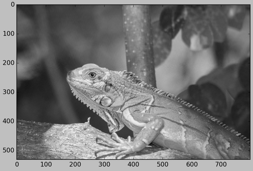
It’s difficult to spot any imperfections or grainy patches in this image, yet it can be stored using less than $2/3$ as much space as the original. This is the beauty of perceptual coding - we’ve actually removed a lot of detail from this image, but it’s so fine that we can barely notice it with the naked eye.
How is it possible to obtain such a good approximation while omitting such a large chunk of the information in the image? To understand why, we have to consider the singular values $\sigma_i$ mentioned earlier. Recall that the terms in the SVD composition are defined by where $\vec{u_i},\vec{v_i}$ have a magnitude of $1$. For some term $E_i$, if the value of $\sigma_i$ is small, then all of the values in the matrix $E_i$ will be relatively small, and omitting $E_i$ from the SVD decomposition will have little impact on the result. Thus, when choosing which terms to omit, it is best to cut out the terms with the smallest $\sigma_i$ values. The smaller these $\sigma_i$ values are in relation to the greater $\sigma_i$ values, the less they will noticeable affect the image quality. Intuitively, we can think of $\sigma_i$ as a measurement of the “importance” or “influence” of $E_i$.
When we SVD decompose a matrix $A$, we list the terms in descending order of $\sigma_i$ magnitude, so that $\sigma_1 >\sigma_2>...\sigma_p$. By summing the first $k$ terms of the SVD decomposition, we are choosing the $k$ terms that are “most important,” or the $k$ terms with the greatest $\sigma_i$ values.
Let’s return to our iguana image. The greatest singular value of this image is equal to $\sigma_1\approx 71,883.3$, while the smallest singular value is $\sigma_{531}\approx 3.26$, so we might say that the most important term in the SVD decomposition is about $20,000$ times as important as the least important term. Here’s a lot plot of the distribution of all of the $\sigma_i$ values:
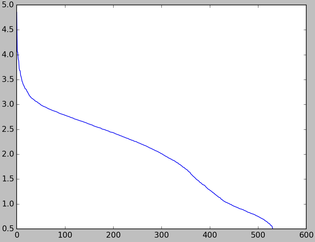
We can see from this graph that very few of the singular values are greater than $10^3$, while more than half are under $10^{2.5}$. Since the greatest singular values are orders of magnitude greater than the smallest, truncating the SVD expansion after the first $200$ terms or so decreases the image quality only slightly.
Before concluding this post, there’s one more cool thing that I’d like to point out. Something interesting happens if we remove the first terms of the SVD decomposition instead of the last terms. Here is the image corresponding to the sum of all terms except the first $20$, or $E_{21}+E_{22}+...+E_{531}$:
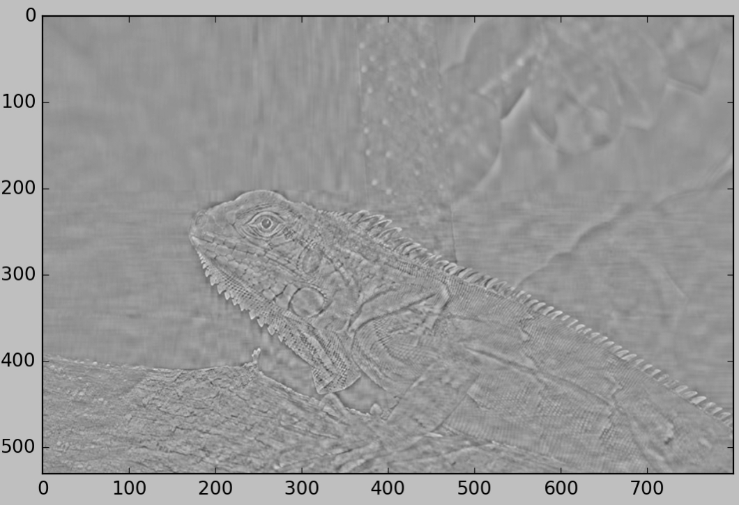
Interestingly, many of the details of the image are still present, and we can certainly tell that it’s supposed to be an iguana. However, only the details are visible - any large patches of light or darkness have been homogenized into a similar bland shade of gray. Only the areas of intricate detail or high-contrast borders between light and dark areas are visible.