Skip to page content Home     Posts     CV     Contact     People

Coproducts and case-splits

In this post, I'd like to discuss a useful concept from category theory that has popped up in several areas of math and computer science that I've studied recently. In particular, this construction can be used to describe:

• Defining a piecewise function on a set
• The analogue of an if-else case switch in Agda or Haskell
• Whether a topological space is connected or disconnected
• The outcome of measuring a qubit or a quantum system

As is often the case, category theory suggests interesting analogies between these different mathematical settings that probably wouldn't have occurred to me otherwise.

Universal property of the sum

Intuitively speaking, the sum or coproduct of objects in a category abstracts the mechanism by which we construct "piecewise" functions in a classical setting like $\mathsf{Set}$, the category of set functions, or in a functional programming language. In $\mathsf{Set}$, we often define piecewise functions $h:A\to B$ in terms of two other functions $f,g:A\to B$, writing something like "define $h(a)$ to be $f(a)$ if $P(a)$ is true, and $g(a)$ if $P(a)$ is false". Or perhaps if $A'\subset A$ is a subset of interest, we might say "define $h(a)$ to be $f(a)$ if $a\in A'$ and $g(a)$ if $a\notin A'$". Notice that for this latter construction, $f$ need not be defined on all of $A$, but only needs to be defined $A'\to B$, and similarly $g$ only needs to be defined $A\backslash A'\to B$.

But these two ways of defining piecewise functions describe $h$ in terms of the values it takes at individual arguments, and in category theory this is a no-no. Good categorical definitions should usually treat objects as black-boxes, performing constructions by leveraging objects' relationships (morphisms) with other objects, rather than their internal structure. Defining morphisms purely in terms of their values at specific elements is especially bad when it comes to generalizing a construction to categories other than $\mathsf{Set}$. It happens to be true in $\mathsf{Set}$ that a function $f:x\to y$ is uniquely determined by its composites $f\circ e$ where $e$ ranges over all "elements" $e:\mathbf 1 \to x$, but this is not true in all categories, nor even in all topoi, which are generally considered to be the most "set-like" categories. (The topoi for which this does hold are called well-pointed topoi.)

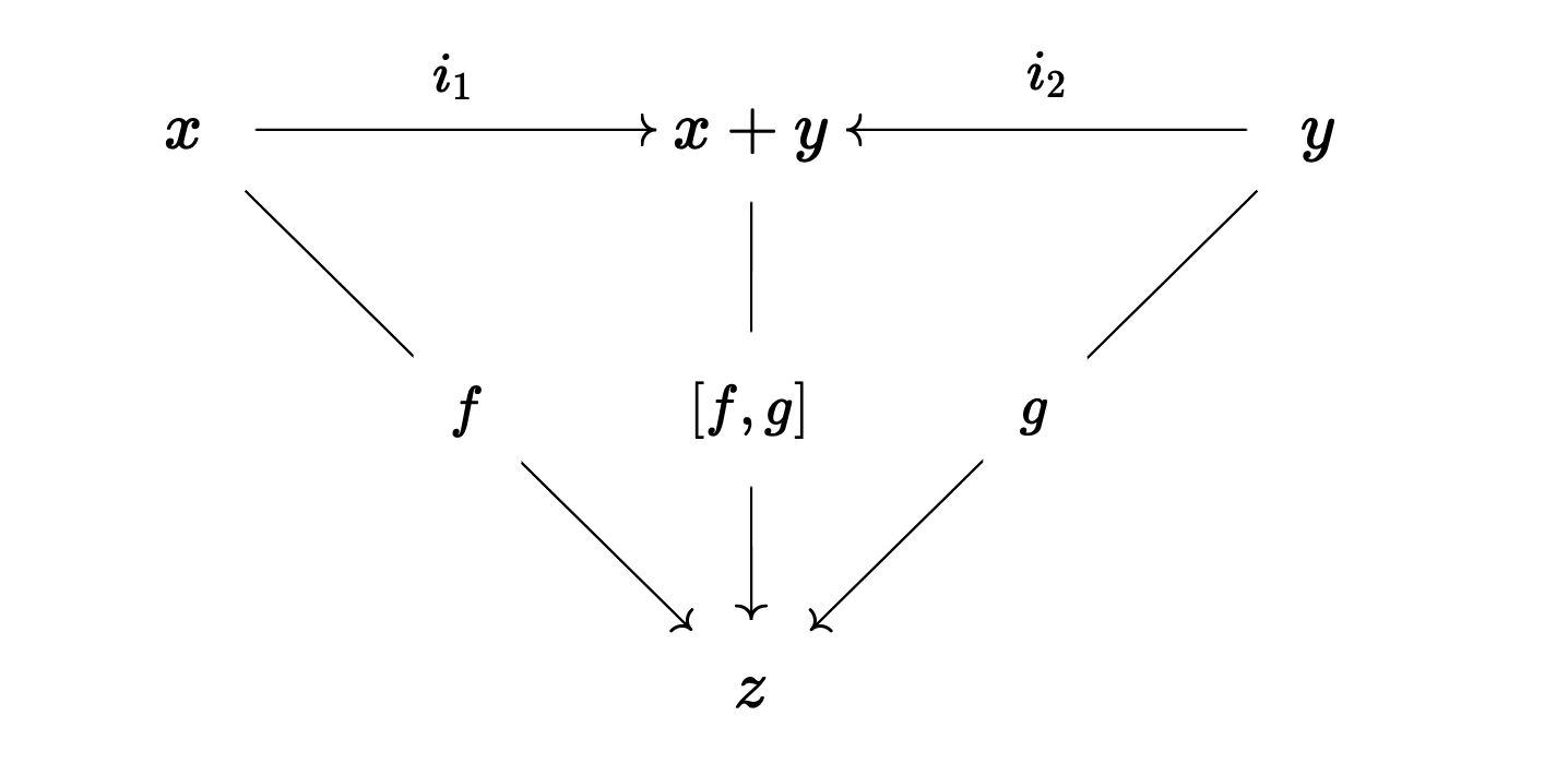
This is the motivation behind the coproduct. Now, here's the technical definition. If $x,y$ are two objects in a category $\mathsf C$, then a coproduct of these two objects is another object, which we will denote $x+y$, such that there are two "inclusion maps" $i_1:x\to x+y$ and $i_2:y\to x+y$ with the property that for any other object $z$ in the category and any two morphisms $f:x\to z$ and $g:y\to z$, there exists a unique arrow $[f,g]:x+y\to z$ satisfying the equations $$[f,g]\circ i_1 = f ~ ~ ~ ~ ~ [f,g]\circ i_2 = g$$ that is, a unique arrow $[f,g]$ making the following diagram commute:

Let's break down this complicated definition a little bit. A coproduct of $x$ and $y$ can kind of be thought of as an object with two "pieces", one piece that "looks like $x$" and another piece that "looks like $y$". Any morphism $h:x+y\to z$ originating from the coproduct $x+y$ can be "restricted" to either of these two pieces by pre-composing with either of the respective inclusion morphisms $i_1$ and $i_2$, giving us either a morphism $h\circ i_1 : x\to z$, telling us how $h$ behaves on the "left side" of the coproduct, and a morphism $h\circ i_2:y\to z$, telling us how $h$ behaves on the "right side" of the coproduct. Not only does the definition of the coproduct tell us this, but it also tells us that these two composites $h\circ i_1$ and $h\circ i_2$ completely determine the behavior of $h$, and that they are independent in the sense that they can be any pair of morphisms $x\to z$ and $y\to z$. In some sense, $x$ and $y$ are included in the coproduct $x+y$ in such a way that they span it completely, together determining the behavior of all outgoing functions, yet are independent or separate from each other, since the behavior of a morphism on one half of the coproduct has no bearing on its behavior on the other half.

In the category of sets $\mathsf{Set}$, any pair of objects $X,Y$ has a coproduct, namely their disjoint union $X\sqcup Y$. The pairing $[f,g]$ of functions $f:X\to Z$ and $g:Y\to Z$ can be defined using precisely the piecewise function construction mentioned earlier. A function originating from $X\sqcup Y$ is determined precisely by the values it takes on $X$, and the values it takes on $Y$, and nothing more. To take another example that might be familiar, in this previous post I worked with coproducts in the type theory of the Agda programming language. In this system, the construction of pairing of two functions $[-,-]$ goes by the name +-recursion. This is the mechanism by which we carry out the equivalent of an if-else case split in Agda.

Notice that coproducts are not necessarily unique, and in fact they are often not unique. For instance, if $X,Y$ are two sets with, say, cardinalities of $|X| = 2$ and $|Y| = 3$, then any set $Z$ with cardinality $5$ is actually a coproduct of $X$ and $Y$, and any injections $i_1:X\to Z$ and $i_2:Y\to Z$ with disjoint images can serve as the inclusion maps. It is, however, true that any two coproducts of a pair of objects in some category $\mathsf C$ must necessarily be isomorphic. So when we write $x+y$ for two objects $x,y$ of a category with coproducts, we are really referring to some possible coproduct of $x$ and $y$, or perhaps a particular object serving as a coproduct of $x$ and $y$ that is understood from context. Our previous example confirms the uniqueness of coproducts up to isomorphism, as any two sets with five elements are isomorphic.

In fact, we can say something a little stronger than "coproducts are unique up to isomorphism". Namely, coproducts are unique up to a unique isomorphism. That is, if $x,y$ are objects of $\mathsf C$ with two distinct coproducts $z,z'$ with respective inclusion maps $i_1,i_2$ and $i_1',i_2'$, then not only can we say that there exists an isomorphism $e:z\simeq z'$, but also that there exists a unique isomorphism $e$ which respects the inclusion maps of the coproduct, that is, with the property that $e\circ i_1 = i_1'$ and $e\circ i_2 = i_2'$. If you want, you can try proving this directly from the definition of the coproduct- it's a fun puzzle and a good way to learn how to use the definition.

This categorical definition of coproducts, although it may feel foreign to someone who is used to classical math and set theory (like me), has the benefit that once you understand it well, it generalizes to many other categories. And unlike in $\mathsf{Set}$, where the classical definition of a disjoint union in terms of elements is probably easier to understand than the categorical definition of a coproduct, this standardized definition may actually help us gain intuition for mathematical objects that are less familiar to us. In the following two sections, I'll describe coproducts in two more exotic categories - $\mathsf{Top}$, the category of continuous functions between topological spaces, and $\mathsf{FinVect}_{\mathbb C}$, the category of finite-dimensional complex vector spaces, which is one possible mathematical stage for the theory of quantum computing. Perhaps more surprising than the fact that these categories have coproducts is the fact that these coproducts can also be interpreted as a way of formalizing if-else case splits, even though it's difficult to see at first glance how these categories have anything at all to say about computation.

Topological spaces and computation

Now I'd like to talk about what the categorical sum construction looks like in $\mathsf{Top}$, the category whose objects are topological spaces and whose morphisms are continuous functions between topological spaces. In what follows, I'll assume some familiarity with the definition of a topology, and how this definition is usually derived as an abstraction of the properties of a metric space.

The intuition for what a topological space means doesn't necessarily need to be spatial or geometric. In fact, the most compelling intuitive understanding I've been able to find for some of the wackier and harder-to-visualize topological spaces out there has come from the ideas described in this MSE post. According to this framework, an open set should be conceptualized not as formalizing some notion of spatial closeness, but rather a notion of computability. In particular, an open subset $U$ of a topological space $X\supset U$ should be thought of as a "semidecidable" subset of $X$, that is, a subset to whom membership can be computationally verified in a finite amount of time.

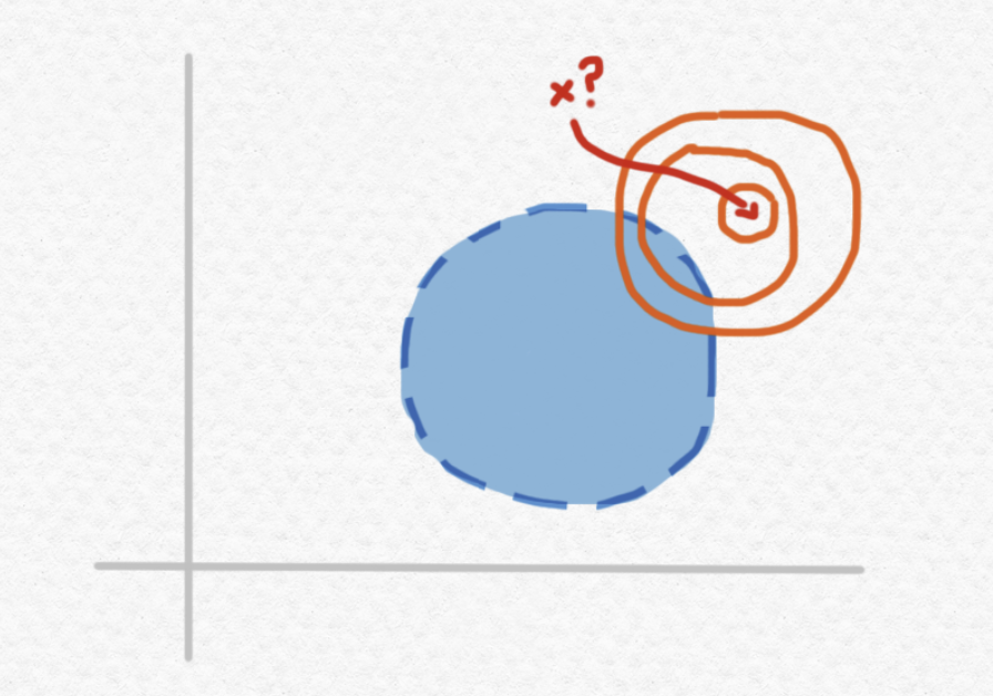
In order to better understand this idea, let's go back to the idea of a metric space like $\mathbb R^2$. Consider an open ball $B\subset \mathbb R^2$ and some point inside of that open ball:

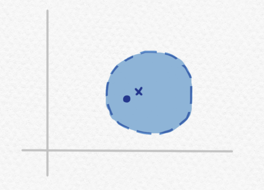
Imagine that we are given a description of the open set $B$ and a description of the point $x$, and tasked with deciding whether or not $x$ belongs to $B$. Since it would take an infinite amount of information (say, decimal digits) to completely specify an arbitrary real number, clearly we can't necessarily know exactly what real number the point $x$ is, even if we're told how to construct it. We could construct increasingly precise approximations of the real number $x$, but the more accurate our approximation, the more time we will need to compute that approximation, and the more memory we'll need to store it. So the above visualization is actually kind of misleading. Rather than imagining that we are given the exact position of the point $x$, we should imagine that we are instead able to calculate smaller and smaller neighborhoods of $x$, representing regions to which we know $x$ belongs based on approximations we've made with greater and greater guarantees of precision:

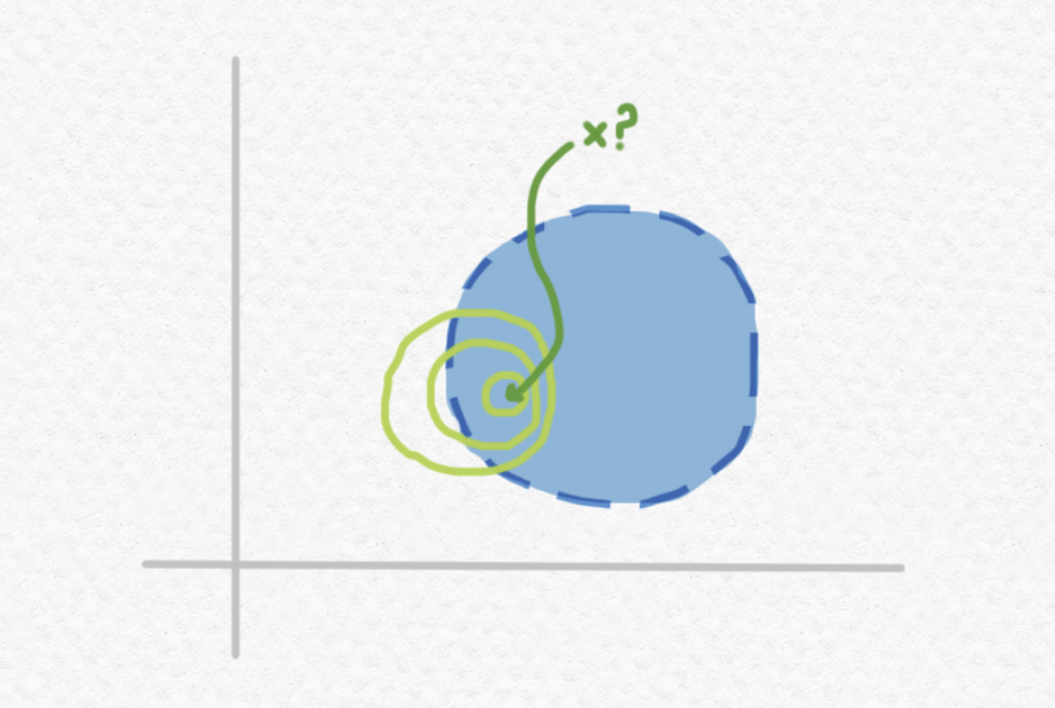
This might seem like a big problem, but if all we want to know is whether $x$ belongs to $B$, we don't actually need to know the exact value of $x$. For instance, in the above picture, knowing that $x$ resides in the smallest of the three pictured neighborhoods would be sufficient to deduce that $x$ does indeed belong to $B$, even though this information still leaves infinitely many possibilities for the exact value of $x$.

Let's express this same point a little more rigorously. Say $B$ is an open ball of radius $r$ about some center point $c$ in a metric space $(X,d)$, that is, it's the set of all points $x$ satisfying $d(x,c) < r$. Further, suppose $x_0\in X$ is some point and that we would like to know whether $x_0$ belongs to $B$ or not. If $x_0$ does in fact belong to $B$, then $d(x_0,c) < r$, or in other words $$r - d(x_0, c) > 0$$ Imagine that given enough time, we are able to compute an approximation of $x_0$ that is guaranteed to have accuracy $\epsilon$ for any $\epsilon > 0$, given a sufficient amount of computational time and memory with which to do so. Then if we carry on computing better and better approximations for $x_0$, so that $\epsilon\to 0$ as we spend more and more time computing better and better approximations, eventually we will come up with an approximation satisfying $$\epsilon < \frac{r-d(x_0,c)}{2}$$ Let's call this approximation $\tilde{x_0}$, so that we know $$d(x_0, \tilde{x_0}) < \frac{r-d(x_0,c)}{2}$$ Well, if we are able to verify that the unknown value $x_0$ falls within this radius of the known value $\tilde{x_0}$, then we would be able to explicitly calculate $d(\tilde{x_0}, c)$ and use this to upper-bound the distance between $d(x_0,c)$ using the triangle inequality, and conclude that $$d(x_0,c) \leq d(x_0,\tilde{x_0}) + d(\tilde{x_0}, c) < \frac{r - d(x_0, c)}{2} + \frac{r + d(x_0, c)}{2} = r$$ and hence verify that $x$ does indeed belong to the ball $B$, despite still not knowing its exact value. To summarize - if $x$ belongs to an open ball $B$, then we will always be able to eventually verify that it belongs to that ball, although we may need more precision to make this determination for some points than for others.

But what about the case in which the given point $x$ happens to not belong to the ball $B$? For instance:

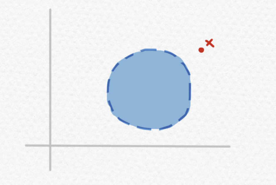
In the particular case depicted above, we can still solve the problem given enough time to compute a sufficiently good approximation of $x$. For instance, if we are able to verify the membership of $x$ to each of the following increasingly small regions through a sequence of approximations:

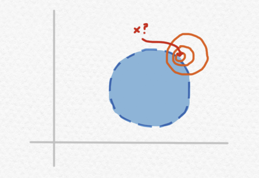
then by the time we obtain the third approximation, we'll be ready to conclude that $x\notin B$, because the region that we know $x$ must belong to has no overlap with $B$. However, what if the point we're given lies on the edge between the interior of $B$ and the exterior of $B$, i.e. on the frontier of the ball $B$?

Note that this point is not actually included in the ball, since the open ball $B$ does not include its circumference. Unlike the previous example, no matter how precise our approximation of $x$, there will always be some "possible values" lying outside of $B$ and other "possible values" lying inside of the circle:

So, no matter how long we continue to approximate $x$, our results will always be inconclusive. This is what is meant by saying that $B$ is a "semidecidable set" - for points that are in fact elements of $B$, we can always verify their elementhood with a finite amount of computation, but for points that are not elements of $B$, this may or may not be possible.

We've determined that an open set $U\subset X$ consists of a set whose members can be verified, so it follows that a closed set $C\subset X$ (the complement of an open set) consists of a set whose non-members can be verified. These properties are not mutually exclusive - it's possible for a subset of a topological space to be both closed and open, and such subsets are (somewhat humorously) called clopen. Under the computational interpretation, these are decidable subsets of $X$, i.e. subsets with the property that we can always decide in a finite amount of time whether any given point of $X$ belongs to that subset or not. Notice that, computationally speaking, being able to decide both membership and non-membership of a subset $A\subset X$ is precisely what we need to compute a case split statement taking the form "if $x$ belongs to $A$, then return $f(x)$, else return $g(x)$". That is, if our computational domains are represented as topological spaces, case-splitting on whether or not a point $x$ satisfied a given property $P$ is not a trivial task and is not even necessarily possible unless the set of points satisfying $P$ is a clopen set. A clopen set of $X$ can also be thought of as a way of decomposing the space into two pieces. Having nontrivial clopen sets is equivalent to being a disconnected topological space, or alternatively having a non-constant map into the discrete topological space with two elements. This map could be interpreted computationally as an "indicator function" for the property $P$.

The punch line is that this is the same as $X$ being homeomorphic to the direct sum of two nonempty topological spaces, $X\simeq X_1 + X_2$. Hence, the universal property of the sum also captures the essential nature of what it means to do a case-split in the category of topological spaces - it just might be a bit trickier to find the ways in which a topological space can be decomposed as a sum, as opposed to a set.

You might be thinking that our prior example using $\mathbb R^2$ is out of touch with what computation involving real numbers looks like in practice. After all, when we write code to do computations involving real numbers, we use case splits all the time. But $\mathbb{R}^2$, endowed with the Euclidean topology, is a connected topological space, meaning that it shouldn't be possible to perform any nontrivial case splits on this domain at all! So what gives?

Well, when we do math with "real numbers", what we're usually working with are floating point numbers of a certain fixed precision. For that reason, the space of floating point numbers, expressed as a topological space, would just carry the discrete topology on a really, really large underlying set. In principle, any set-function from the floating point numbers to any other set should be realizable - it might just take a really long time to write out all of the cases. A data type representing real numbers more faithfully might look something like a type of streams of digits which lazily produces digits of precision on demand. (Cardinality and computability issues still prevent this kind of representation from being an honest-to-god implementation of the real numbers as they are defined set-theoretically, but it's a lot better than floating point numbers.)

But a computational representation of the real numbers in which no case splits are possible sounds horrific. How could we do any kind of meaningful computation on a doman where we can't use case splits?

One possibility that occurs to me would be to work primarily with partial functions on $\mathbb R$ or other connected domains, that is, functions that are defined only on a subset of the original space, or functions that are allowed to be "undefined" at certain values. Suppose, for instance, that we wanted to define a piecewise function on $\mathbb R^2$ that behaves one way on the interior of the unit circle and another way on the rest of $\mathbb R^2$ (including both the circumference and the exterior of the unit circle). This is, of course, impossible, since $B(0,1)$, the interior of the unit circle, is not clopen. However, if we use $\mathbb R^2\backslash \mathbb S^1$ (with the induced subspace topology) as the domain of our function, this will be possible, since "cutting out" the circumference of the unit circle turns the plane into a disconnected topological space onto which we can perform the desired case split:

Of course, this comes at the cost of defining our piecewise function not on all of $\mathbb R^2$ but rather only on "most" of $\mathbb R^2$. Another alternative would be to add an extra element to the codomain of our function which represents the possibility of "no output" or "running forever". That is, if the desired output type of our function is represented by the topological space $(Y,\mathcal S)$, then we can modify this space as follows: $$(Y\cup \{\bot\}, \mathcal S \cup \{Y\cup\{\bot\}\})$$ That is, we augment the original space with this additional "no output" point $\bot$, and add only a single open set to the topology consisting of the entire space. This has the consequence that the result $\bot$ computationally cannot be distinguished from any of the legitimate output values, since the only open set containing it is the entire space. This makes sense intuitively: if a function runs forever when evaluated at a specific argument, no matter how long you sit and watch it run, there remains the possibility that it's just about to finish and return an actual value.

Quantum measurements as sums

We've just seen how modeling computability using topological spaces places some restrictions on the "case splits" that can be performed, unlike in $\mathsf{Set}$, where any partition of a set into two pieces is fair game. Now let's look at another category that complicates the ability to perform case splits, this time due to the laws of physics. The category in question is $\mathsf{FinVect}_{\mathbb C}$, the category of finite-dimensional vector spaces over $\mathbb C$. While objects of $\mathsf{Set}$ might be used to model sets of possible states of a classical computer or piece of information - for instance, using ${0,1}$ to represent the set of possible states of a single bit - the objects of this new category represent spaces of possible states occupied by a quantum system.

A qubit is a quantum system whose state corresponds to an element of complex projective space of two dimensions, $\mathbf{P}(\mathbb C^2)$. The possible states of a qubit can be represented as unit vectors in $\mathbb C^2$, with the hitch that two unequal complex unit vectors of dimension two that are linearly dependent (differ by a factor of $e^{i\theta}$) actually represent the same quantum state.

Physically, the state of a qubit cannot be directly observed, that is, given a qubit in some unknown mystery state $\lvert \psi\rangle$ there is no way to determine its state for certain, nor even approximate it to an arbitrary degree of accuracy. The only way to extract information from a quantum system is to perform a measurement on it. Measurements on quantum systems are (thought to be) inherently probabilistic - that is, some measurements produce nondeterministic results not due to errors in our measuring devices, but because the result inherently cannot be known before the measurement is performed. (If you're curious about how this hypothesis could possibly be tested scientifically, read about local hidden-variable theories and Bell's theorem.)

Suppose the state of a qubit is described by the following unit vector: $$\lvert \psi\rangle = \alpha\lvert 0\rangle + \beta\lvert 1\rangle$$ where $\lvert 0\rangle$ and $\lvert 1\rangle$ denote the two standard basis vectors of $\mathbb C^2$, and $\alpha,\beta\in\mathbb C^2$ are such that $|\alpha|^2 + |\beta|^2 = 1$, since this is a unit vector. Measuring this state can result in one of two possible outcomes: either $\lvert 0\rangle$, which occurs with probability $|\alpha|^2$, or $\lvert 1\rangle$, which occurs with probability $|\beta|^2$. Hence, states with a greater component in the $\lvert 0\rangle$ direction are more likely to produce that result when measured, and similarly for $\lvert 1\rangle$, and the states $\lvert 0\rangle$ and $\lvert 1\rangle$ themselves actually produce deterministic results when measured this way. Furthermore, after the qubit is measured, its state will "collapse" to the result of the measurement. If the outcome of the measurement is $\lvert 0\rangle$, then the qubit's state will be changed to $\lvert 0\rangle$ as a result to the measurement, and similarly to $\lvert 1\rangle$. Therein lies the difficulty of extracting information about the qubit's initial state - it's not possible to extract information about a quantum system's state without also changing that state.

Actually, this is not the only possible way to measure a qubit. The standard basis ${\lvert 0\rangle, \lvert 1\rangle}$ is just one of many possible bases with respect to which a measurement can be made. If the state $\lvert\psi\rangle$ is expressed in terms of a different orthonormal basis ${\lvert v_0\rangle, \lvert v_1\rangle}$ of $\mathbb C^2$: $$\lvert\psi\rangle = \alpha' \lvert v_0\rangle + \beta'\lvert v_1\rangle$$ we may also perform a measurement with respect to this different basis ${\lvert v_0\rangle, \lvert v_1\rangle}$, which similarly produces one of two possible outcomes $\lvert v_0\rangle$ and $\lvert v_1\rangle$, with respective probabilities equal to the magnitudes of $\lvert \psi\rangle$ in these two directions, after which $\lvert\psi\rangle$ collapses into the basis state that was observed.

This leads to some very curious behavior. Consider, for instance, the following two quantum states, which form an orthonormal basis for $\mathbb C^2$, sometimes known as the Hadamard basis: $$\lvert +\rangle = \frac{\lvert 0\rangle + \lvert 1\rangle}{\sqrt{2}} ~ ~ ~ ~ ~ \lvert -\rangle = \frac{\lvert 0\rangle - \lvert 1\rangle}{\sqrt{2}}$$ Since the components of these states are purely real we might picture them as vectors on the unit circle in $\mathbb R^2$:

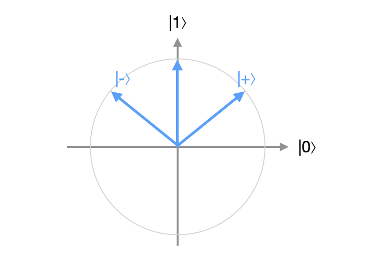
If we measure $\lvert +\rangle$ with respect to the standard basis ${\lvert 0\rangle, \lvert 1\rangle}$, we will obtain the result $\lvert 0\rangle$ about $50\%$ of the time and the result $\lvert 1\rangle$ about $50\%$ of the time, since $\alpha=\beta=1/\sqrt{2}$ gives $|\alpha|^2 = |\beta|^2 = 0.5$. On the other hand, measuring $\lvert -\rangle$ with respect to the standard basis also gives both results with a probability of $50\%$, since $\alpha=-\beta=1/\sqrt{2}$ also gives $|\alpha|^2 = |\beta|^2 = 0.5$. So if we were given one of these two states without knowing which, we wouldn't be able to tell any difference between them at all by measuring in the standard basis - in both cases, the measurement result would act like a fair coin flip. But measure the state in the basis ${\lvert +\rangle, \lvert -\rangle}$ and the outcome of our measurement will tell us exactly which state the qubit is in. Conversely, measuring a mystery qubit in one of the two standard basis states with respect to ${\lvert +\rangle, \lvert -\rangle}$ will give us coin-flip-like results that gives us no information about the qubit's state.

This measurement rule is not restricted to qubits, which occupy a state space of only two dimensions. Generally speaking, we can consider the $\mathbb C^n$, in which the computational basis (or any other basis) has exactly $n$ elements. For instance, a qutrit is a quantum system whose state occupies the space $\mathbb C^3$. A quantum state space does not even need to be finite-dimensional, so long as it is a Hilbert space.

In a state space with more than two dimensions, the result of a measurement need not completely determine the end state of a system, either. More generally, a projection valued measure on a finite dimensional complex Hilbert space $\mathbb C^n$ consists of a sequence of projection operators $P_1,\cdots,P_k$ onto mutually orthogonal subspaces that span all of $\mathbb C^n$. The possible outcomes of the measurement correspond to the projectors $P_1,\cdots,P_k$, the probability of obtaining the outcome $P_j$ when measuring the state $\lvert \psi\rangle$ is equal to the squared magnitude $\lVert P_j\lvert \psi\rangle\rVert^2$ of the component of that vector in the space corresponding to $P_j$, and after observing such a result, the system "collapses" into the state parallel to its component in that subspace.

To take another example, consider the state space $\mathbb C^3$ of qutrits, and suppose that we have a qutrit in the following state: $$\lvert\psi\rangle = \frac{\lvert 0\rangle + \lvert 1\rangle + \lvert 2\rangle}{\sqrt{3}}$$ A full measurement with respect to the standard basis ${\lvert 0\rangle, \lvert 1\rangle, \lvert 2\rangle}$ would produce one of three possible equally likely outcomes, each with probability $1/3$. This measurement could be expressed as a projective measurement in which the projectors are given by $$\begin{align*}P_0 &= \lvert 0\rangle\langle 0\rvert \\ P_1 &= \lvert 1\rangle\langle 1\rvert \\ P_2 &= \lvert 2\rangle\langle 2\rvert\end{align*}$$ These are the projection operators that project vectors onto each of the three respective coordinate axes, which are one-dimensional subspaces of $\mathbb C$. However, we could also perform a projective measurement corresponding to the following two projectors: $$\begin{align*}P_0 &= \lvert 0\rangle\langle 0\rvert \\ P_1 &= \lvert 1\rangle\langle 1\rvert + \lvert 2\rangle\langle 2\rvert\end{align*}$$ If we measure $\lvert\psi\rangle$ according to this projective measurement, we would either receive the outcome $P_0$ with probability $1/3$, in which case the qutrit would collapse into the state $\lvert 0\rangle$, or the outcome $P_1$ with probability $2/3$, in which case the qutrit would collapse into the state $\tfrac{1}{\sqrt{2}}\lvert 1\rangle + \tfrac{1}{\sqrt 2}\lvert 2\rangle$. Notice that if we did not know the initial state of this qutrit, after receiving a result of $P_0$ we would know its exact state, but after receiving a result of $P_1$, we would not know its exact state, only that this state lies in the two-dimensional subspace spanned by $\lvert 1\rangle$ and $\lvert 2\rangle$.

The topic of quantum measurements is really complicated, and I wouldn't expect to be able to do it justice in this blog post. We haven't even touched on many fascinating and mind-bending phenomena like interference and entanglement. I'd encourage you to read more about this elsewhere if it interests you - I like the book Quantum Computation and Quantum Information by Nielsen and Chuang, and my quantum computing class at the Universidad de Granada has used the book Quantum Information Processing by Bergou and Hillery. But wait a minute - what does any of this have to do with category theory and coproducts?

Well, as we've discussed, $\mathsf{FinVect}_{\mathbb C}$, the category of finite-dimensional complex vector spaces with linear transformations as its morphisms, is a pretty decent mathematical setting for studying quantum systems and measurements. As you might have guessed, this category has coproducts. The coproduct of two complex vector spaces $V,W$ is their direct sum, denoted $V\oplus W$, which is often defined as the vector space whose elements are pairs of vectors $(\mathbf v,\mathbf w)$ - one element from $V$ and one element from $W$ - such that vector addition and scalar multiplication is defined elementwise. That is, $$(\mathbf v_1, \mathbf w_1) + (\mathbf v_2, \mathbf w_2) = (\mathbf v_1+ \mathbf v_2 , \mathbf w_1 + \mathbf w_2)$$ and $$\alpha\cdot (\mathbf v, \mathbf w) = (\alpha\cdot \mathbf v, \alpha\cdot \mathbf w)$$ The inclusion maps $i_1:V\hookrightarrow V\oplus W$ and $i_2:W\hookrightarrow V\oplus W$ are defined as follows: $$\begin{align*}i_1 ~ &: ~ \mathbf v\mapsto (\mathbf v, \mathbf 0) \\ i_2 ~ &: ~ \mathbf w \mapsto (\mathbf 0, \mathbf w)\end{align*}$$

Notice that this is a little different than the examples of coproducts we've seen so far in $\mathsf{Set}$ and $\mathsf{Top}$. In particular, when we took a coproduct of two sets or topological spaces, each element of the coproduct directly corresponded to an element of one of the two sets or spaces being added together. That is, each element of the coproduct was an inclusion from either the left half or the right half of the coproduct. This is not the case for coproducts of vector spaces. If $\mathbf v$ and $\mathbf w$ are both nonzero, then the vector $(\mathbf v, \mathbf w)$ of the coproduct space $V\oplus W$ is not the inclusion of a vector from either space. It can, however, be expressed as a sum of included vectors by writing $$(\mathbf v, \mathbf w) = (\mathbf v,\mathbf 0) + (\mathbf 0, \mathbf w)$$ and this fact is the key to seeing why $\oplus$ satisfies the requirements of a coproduct. For if $h:V\oplus W\to X$ is a morphism of $\mathsf{FinVect}_{\mathbb C}$, that is, a linear transformation, and the morphisms $f:V\to X$ and $g:W\to X$ describe how it acts on vectors of the form $(\mathbf v, \mathbf 0)$ and $(\mathbf 0, \mathbf w)$, then the linearity of $h$ determines its values at all elements of $V\oplus W$, even those that are not included from either $V$ or $W$: $$\begin{align*}h\big((\mathbf v,\mathbf w)\big) &= h\big((\mathbf v,\mathbf 0) + (\mathbf 0,\mathbf w)\big) \\ &= h\big((\mathbf v,\mathbf 0)\big) + h\big((\mathbf 0,\mathbf w)\big) \\ &= f(\mathbf v) + g(\mathbf w)\end{align*}$$

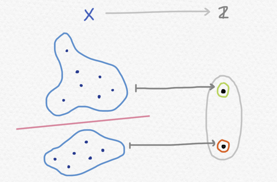
Now, here's the connection. Suppose that $V$ is the space of states of some quantum system, and that we've defined a projective measurement on $V$ according to two projection operators $P_0,P_1$, so that the measurement has two possible outcomes. Then $P_0$ and $P_1$ project onto two different subspaces $V_0,V_1\subset V$, and these subspaces are mutually orthogonal. This means that every vector $\mathbf v\in V$ can be decomposed uniquely as a sum of its components in each space $\mathbf v = \mathbf v_0 + \mathbf v_1$. Consequently, we might identify vectors in $V$ with pairs of components in each of these two subspaces, leading us to conclude that $$V \simeq V_0 \oplus V_1$$ that is, the whole space $V$ is isomorphic to the direct sum of its two mutually orthogonal subspaces. See what's going on here? Describing a measurement on a quantum system with state space $V$ essentially boils down to describing $V$ as a coproduct of two smaller spaces.

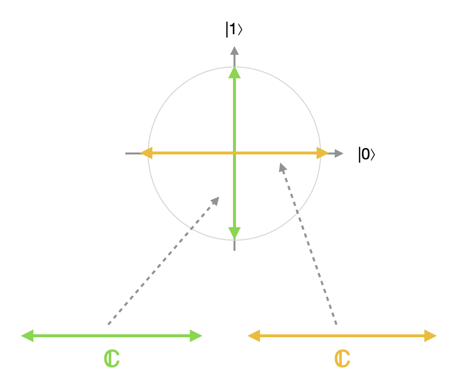
The point we made earlier about coproducts being non-unique is really important in this example. For instance, the two-dimensional complex vector space $\mathbb C^2$ is a coproduct of $\mathbb C^1$ and $\mathbb C^1$, but there are many different possible inclusion maps $i_1,i_2:\mathbb C^1\to \mathbb C^2$ that will satisfy the coproduct laws, and these different inclusions correspond to measurements with respect to different bases. For instance, a measurement in the computational basis ${\lvert 0\rangle, \lvert 1\rangle}$ would correspond to a decomposition of $\mathbb C^2$ into a coproduct $\mathbb C\oplus\mathbb C$ with the following inclusions:

whereas a measurement in the Hadamard basis ${\lvert +\rangle, \lvert -\rangle}$ would correspond to a coproduct decomposition with the following inclusions:

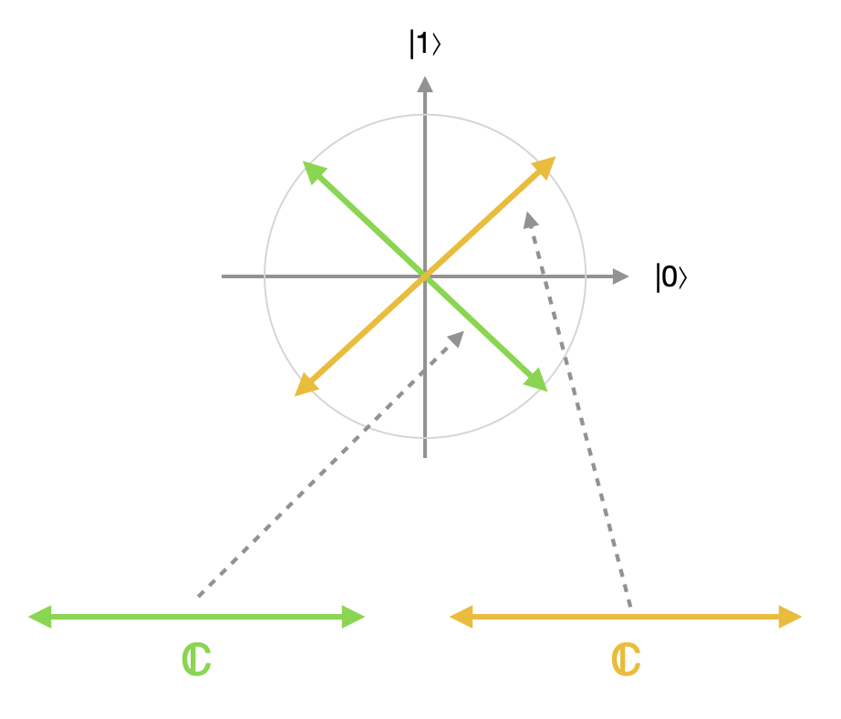
Distinguishing between the different ways of expressing $\mathbb C^2$ as a coproduct of $\mathbb C^1$ and $\mathbb C^1$ in this context is pretty important. Depending on which state we're measuring, the difference between these two coproduct representations, or measurements in two different bases, could be as stark as the difference between completely deterministic behavior and a 50-50 coin flip. There's a whole continuum of possible coproduct decompositions of $\mathbb C^2$. As a matter of fact, the space of all possible orthonormal bases for $\mathbb C^2$ can be endowed with a natural topology making it homeomorphic to two-dimensional real projective space $\mathbf{P}(\mathbb R^2)$.

Finally, this example of the coproduct also expresses something about the peculiar nature of classical case-splits in quantum computation. In essence, the only way we can force a classical dichotomy onto a quantum system is to perform a measurement and base what we do next on the result of that measurement. If we want to design an algorithm that reliably behaves one way on one kind of state and behaves a different way on another kind of state, as if we were defining a piecewise function, those two classes of states had better lie in orthogonal subspaces - and any states lying in between, with nonzero components in both subspaces, will give rise to nondeterministic behavior.

Sum food for thought

Here are a couple of fun problems to think about:

1. Consider the functor category $\mathsf{Set}^{\mathbb N}$ of "sets through time", as described at the end of this previous post.

   • Show that this category has coproducts.
   • If a set is "disconnected", i.e. is isomorphic to a sum of two nonempty sets, at each instant in time, then is it necessarily disconnected for all time? That is, if $F:\mathbb N\to\mathsf{Set}$ is an object of this functor category and $Ft\simeq x_1 + x_2$ for some nonempty sets $x_1,x_2$ for all instants $t$ in $\mathbb N$, then is $F\simeq F_1 + F_2$ for some nonempty $F_1,F_2$? (Where "$X$ is nonempty" is defined to mean that there exist "elements" $\mathbf 1 \to X$.) Another way of phrasing this question would be: does being locally disconnected imply being globally disconnected?
   • Consider the previous question in the more general case $\mathsf{Set}^{\mathbb P}$ where $\mathbb P$ is an arbitrary poset. What conditions on the poset $\mathbb P$ are necessary and sufficient for this to be true?

2. It is mentioned in this previous post that if $\mathsf C$ is a category with sums, then for any fixed object $E$ of $\mathsf C$, there is a monad acting on objects by sending $x\mapsto x + E$. Can you define this functor, prove that it satisfies the functor laws, and prove that it satisfies the monad laws using the universal property of the coproduct?

3. Consider a category $\mathsf{Conv}$ whose objects are convex subsets of real vector spaces, and whose morphisms are affine maps, i.e. functions $f:X\to Y$ satisfying $$f\big(r\mathbf x + (1-r)\mathbf y\big) = rf(\mathbf x) + (1-r)f(\mathbf y)$$ for all $r\in [0,1]$. That is, they are functions preserving weighted averages.

   • Verify that this does in fact define a category. The only nontrivial part of this proof is to verify that the composition of affine maps is affine.
   • Does this category have coproducts?