This is the story of how I wrote an absurdly inefficient algorithm to solve a cool problem in R, learned about copy-on-write semantics, and then came up with something much faster. This debacle has definitely made me a better R programmer.
At my job, I’m working with a cyber intrusion dataset from the Canadian Institute for Cybersecurity that contains large lists of flows with associated statistics summarizing the traffic comprising each flow. These include stats like the flow’s total duration, the average rates of data transfer in packets per second and bytes per second, the mean and standard deviation length of a packet, and so on.
A "flow" in this data set is confined to one of three network protocols (TCP, UDP and ICMP) and is identified by a pair of IP addresses identifying the source and destination, a pair of port numbers being used by the source and destination machines respectively, and a window of time distinguishing the flow from earlier and later flows. It happens that for our analysis, we want to aggregate all of the flows with the same source/destination IP and source/destination port and discard the time-based delimitation between flows. To describe the problem more abstractly: given several subsets partitioning a larger population, and a set of statistics for each subset in the partition, we need a way of coming up with the corresponding statistics for the overall population.
Ignoring questions of efficiency, this can be an interesting problem in its own right. Indulge me for a second, and imagine that we’re looking at pieces of summary data collected about a pet shelter during several disjoint observation periods. Each data point might include:
For some types of statistics, the aggregation rule is obvious. For instance, if during an observation period at shelter $X$ the maximum cat intake on a single day was $c_X$, and during an observation period at shelter $Y$ the maximum cat intake on a single day was $c_Y$, then the maximum cat intake over all days included in both observation periods must be $\max(c_X,c_Y)$. More generally, given a vector $\mathbf{c}$ of maximum cat intake values over several observation periods, the overall maximum cat intake could be computed by folding this operation over the vector by computing $\texttt{fold}(0, \text{max}, \mathbf{c})$. And if the number of days in the former observation period is $d_X$ and the number of days in the latter observation period is $d_Y$, then the total number of days is $d_X+d_Y$. Similarly, for a vector of durations $\mathbf{d}$ of several observation periods, the overall duration could be computed as $\texttt{fold}(0, +, \mathbf{d})$.
However, some statistics, such as averages, are not so neat. If the average daily cat intake at during the observation of shelter $X$ was $\mu_X$ and the average daily cat intake during the observation of shelter $Y$ was $\mu_Y$, the average daily cat intake of the combined observation periods could be anywhere between $\mu_X$ and $\mu_Y$, depending on the comparative lengths of the observation periods. If they were equally long, the aggregate average will be $\tfrac{1}{2}\mu_X + \tfrac{1}{2}\mu_Y$, or the average of the averages. But if, for instance, the latter observation period was twice as long, then the aggregate average will be $\tfrac{1}{3}\mu_X+\tfrac{2}{3}\mu_Y$, a weighted average of $\mu_X$ and $\mu_Y$ that favors $\mu_Y$ more heavily. So it’s not even possible to know the aggregate average without another piece of information, namely the duration of the respective observation periods.
This complicates things slightly, but when we have the additional piece of auxiliary data necessary to calculate the aggregate averages, we can do so using a slightly more complex operation that takes more arguments. In particular, given a pair $(d_X,\mu_X)$ containing the duration $d_X$ and the average daily cat intake $\mu_X$ for observation period $X$, and the same pair of statistics $(d_Y,\mu_Y)$ for observation period $Y$, the corresponding pair of statistics for the aggregate collection of days is given by We can reason through this as follows: if $\mu_X$ is the average daily cat intake over period $X$, which lasts $d_X$ days, then the total cat intake over this period is $d_X\mu_X$. Similarly, $d_Y\mu_Y$ is the total cat intake over period $Y$. Hence, their overall average daily cat intake is therefore $d_X\mu_X+d_Y\mu_Y$, the total cat intake, divided by $d_X+d_Y$, the total observation duration. The above defines an associative operation for combining statistic pairs $(d_X,\mu_X)$ and $(d_Y,\mu_Y)$, so if we are given a whole vector $\mathbf{d}$ of durations of $n$ different observation periods and another vector $\boldsymbol{\mu}$ of averages for these respective observation periods, we can compute aggregate statistics by folding this operation over the rows of the $k\times 2$ matrix $[\mathbf{d}\mid\boldsymbol{\mu}]$.
So, what about something even more complicated, like the standard deviation dog adoption per day? For two observation periods $X$ and $Y$, the aggregate standard deviation can’t be computed purely in terms of the respective standard deviations $\sigma_X$ and $\sigma_Y$. It can’t even be computed given the respective durations $d_X,d_Y$ in addition to these statistics. However, given additional data of consisting of the respective durations and the respective average daily dog adoption rates, the aggregate standard deviation can be computed. To be precise, if $(d_X,\mu_X,\sigma_X)$ lists the duration, average dog adoption rate, and standard deviation of dogs adopted per day during observation period $X$, and $(d_Y,\mu_Y,\sigma_Y)$ is analogously defined for period $Y$, then the aggregate statistics are given by As for why this complicated formula works, I’ll leave that as an exercise. If you want a hint, you might find the following fact useful: if $A$ is a random variable, the variance of $A$ (which is the square of its standard deviation) is given by $\text{Var}(A)=\mathbb E[A^2]-\mathbb E[A]^2$.
If you’ve had enough of my contrived example, replace "days" with "seconds", replace "observation period" with "traffic flow", and replace "cat intake" and "number of dogs adopted" with network flow statistics like
My approach starts by identifing which subsets of columns depend on each other for accumulation. Any column collecting a maximum or minimum over the packets in a flow relies only on itself and can be folded using either the maximum or minimum function. Any statistic collecting an average relies on the size of the population being averaged over, and any statistic collecting a standard deviation or variance relies on both the average and the population size.
Now let’s start thinking about optimization. This whole "folding" approach is conceptually helpful, but it would be extremely inefficient to operate on my data this way in R.
First of all, we’ve just seen that aggregating standard deviation data involves computing square roots. Square-rooting is an expensive operation compared to elementary arithmetic operations, and folding such an operation over a matrix with $n$ rows would involve computing square roots $n$ times, even though most of these intermediate values are subsequently squared during the next folding step, making a lot of the square roots superfluous.
Secondly, my data is stored in a dataframe and is hence columnar. This means that the most efficient way to operate on the data is columnwise, and folding an operation over the rows of my dataframe would be the antithesis of this. Not to mention that R can optimize some vector operations that are applied uniformly over vectors, and some of the folding operations described earlier are heterogeneous over columns.
I’m pretty satisfied with this general approach to the problem. For most of the groups of codependent statistics in my dataset, a simple transformation converts them into statistics that are additive, and can hence be aggregated by folding addition over the rows - an operation sufficiently simple and ubiquitous that it’s surely optimized internally.
For instance, suppose that the pair $(d_X, r_X)$ represents the duration and the average per-second rate of packet transmission in a certain flow $X$. Earlier we saw a binary operation for aggregating these stats with the same stats $(d_Y,r_Y)$ for a different flow $Y$ by taking a weighted average of rates, but we will now take a subtly different approach. We can convert the pair of statistics "duration" and "average packet rate" into the pair of statistics "duration" and "number of packets" with no loss of information by mappin $(d,r)\mapsto (d,dr)$, and we can convert these statistics back to the original ones by mapping $(d,n)\mapsto (d,n/d)$. But the latter pair of statistics is additive: the total duration of a collection of flows is just the sum of their durations, and the total number of packets in a collection of flows is just the sum of their packet counts. So if $\mathbf{d}$ is a column vector of duration statistics, and $\mathbf{r}$ is a column vector of rate statistics, then would be the pair of aggregate statistics, where products and quotients are taken elementwise in the above formula. If the data set consists of $n$ rows, we’d only need $3n-1$ floating-point operations to compute the above expression, whereas folding the gnarly weighted averaging operation from earlier would require $6n-6$ FLOPs. Not to mention that this formula uses vectorized operations like the elementwise product and quotient that can be further optimized.
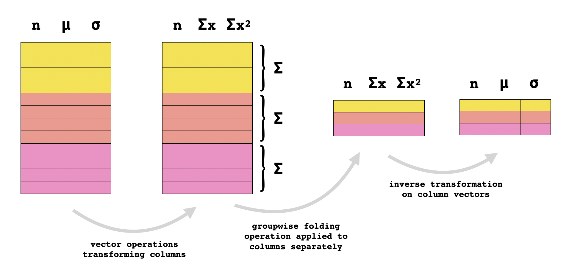
The same trick applies for triples of statistics taking the form $(n,\mu,\sigma)$ where $n$ is the size of some population and $\mu$ and $\sigma$ are the average and standard deviation of some quantitative attribute over that population. These stats aren’t additive, but if we transform them as follows: they become the population size, the sum of the attribute values, and the sum of the squares of the attribute values. And these are all additive, so once the data records are transformed in this way, they can simply be summed together, and then converted back to the original statistics using the inverse transformation:
So, for groups of columns that depend on each other, the algorithm looks like this:
I wrote some code implementing this "optimized" algorithm. It took a couple of days to completely aggregate the grouped flow data. But since then, I’ve written a new version of the algorithm that accomplishes the same in less than five minutes.
So, what the hell happened?
It’s because I didn’t understand how memory management in R works. I forgive myself for this blunder: having never used R for a real project like this before, I didn’t have any foundational knowledge about how it operates under the hood, and I’ve been thrust into learning it quickly. Now, not only do I know how to (sometimes) avoid writing code that takes one thousand times longer than it needs to, but I also find the explanation behind it pretty darn interesting!
The first step is to learn what data structures R uses for its different data types.
Here’s a little bit of terminology, taken straight from the official R Internals guide. A pointer to an object or data structure in memory is called as SEXP, and the actual data structure that it points to is called a SEXPREC. As you go about declaring variables and assigning them values in your R code, the symbols corresponding to the variable names that you choose are associated with SEXPs pointing to the associated data structures in memory. Each SEXPREC has an associated SEXPTYPE, and here are some examples of SEXPTYPE that you might encounter:
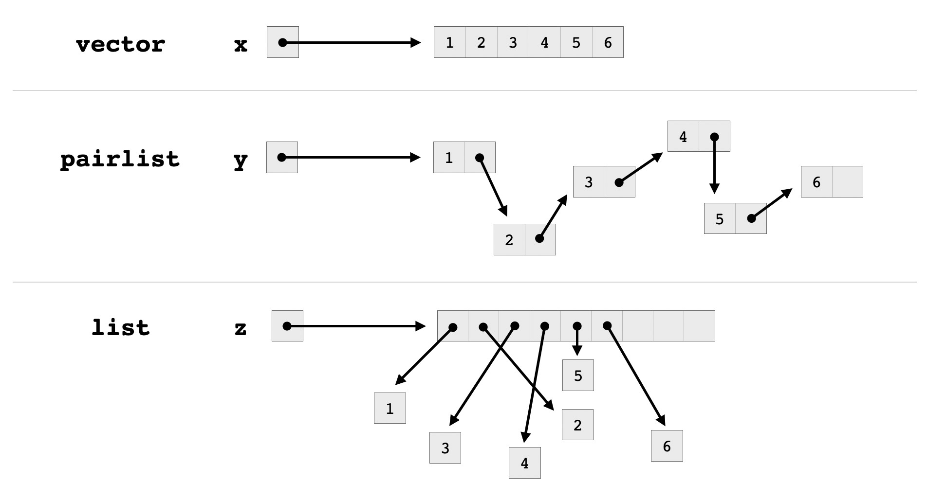
LISTSXP is the type of pairlists.REALSXP is the type of numeric vectors.STRSXP is the type of character vectors.VECSXP is the type of lists.Vectors in R are implemented as C arrays, meaning that they consist of contiguous blocks of memory divided into equally-sized entries containing the same type of data. Pairlists are essentially linked lists, and they actually do not correspond to the list type in R, despite the deceptive SEXPTYPE name LISTSXP. Unlike a linked lists, an R list, which has type VECSXP, consists of a pointer array whose entries point to the respective objects stored in the list. Consequently, accessing an element at a given index of a list requires following fewer pointers than accessing an element at the corresponding index of a pairlist.
An R dataframe is essentially a list of (column) vectors, but with some extra bookkeeping. For instance, dataframes are supposed to have the same number of entries in each column, and the same data type in each column, and the language will enforce this. You can read the source code for R dataframes in this repo. Soon we’ll see how some of this bookkeeping can cause trouble for us, and how an actual list of vectors can serve us better for some use-cases.
Some sources online say that objects in R are immutable: assignment-related idioms of the language merely create the illusion of in-place modification while actually copying objects under the hood. It’s true that this often happens, and that it can seriously degrade performance when it happens unintentionally, but it does not always happen.
R uses copy-on-write semantics for its data structures. This means that when we "copy" a data structure from x to y by executing y <- x, we are really only copying a pointer: the actual data structure in memory is shared by x and y. But when one of x or y is subsequently modified, the data structure is fully copied, and one of the two symbols receives a pointer to the revised copy. R does not copy a data structure upon modification unless multiple references point to it, and reference counters are used to detect such scenarios. This behavior is often (but not always) indistinguishable from what would happen if the data structure were immediately copied, and you could think of copy-on-write as a "lazy copying" mechanism.
The first step in investigating copy-on-write in R is finding a way to actually verify that an object has been copied. For us, this will be the internal function called inspect, which can be used to view useful low-level information about R objects such as their location in memory, their type and their reference counters. I found it difficult to find authoritative documentation on inspect, but this blog post was extremely useful for me when trying to understand its output.
Let’s have a look at what really happens when we perform "assignments" involving a few different data structures in R.
We can create a new real vector and inspect it as follows:
> x <- c(1,2,3)
> .Internal(inspect(x))
@5572a2318d08 14 REALSXP g0c3 [REF(1)] (len=3, tl=0) 1,2,3
From this, we can conclude that we have in fact created a SEXP that points to a SEXPREC of type REALSXP, and we have associated it with the symbol x. Next, we can mutate this vector by setting its first element equal to four, and inspect it again to see what has changed:
> x[1] <- 4
> .Internal(inspect(x))
@5572a2318d08 14 REALSXP g0c3 [REF(1)] (len=3, tl=0) 4,2,3
Note that the memory location 5572a2318d08 did not change at all. This indicates that x was not copied, but rather mutated in-place. Note that this doesn’t contradict the copy-on-write paradigm. The real vector at location 5572a2318d08 wasn’t being referenced by multiple different symbols, as evidenced by the reference counter REF(1), and copy-on-write only demands that copies be made when writing to shared resources. Look at what happens when we "copy" this vector to another variable y, and then attempt to mutate it.
> y <- x
> .Internal(inspect(x))
@5572a2318d08 14 REALSXP g0c3 [REF(2)] (len=3, tl=0) 4,2,3
> .Internal(inspect(y))
@5572a2318d08 14 REALSXP g0c3 [REF(2)] (len=3, tl=0) 4,2,3
> x[1] <- 5
> .Internal(inspect(x))
@5572a2318a88 14 REALSXP g0c3 [REF(1)] (len=3, tl=0) 5,2,3
> .Internal(inspect(y))
@5572a2318d08 14 REALSXP g0c3 [REF(1)] (len=3, tl=0) 4,2,3
Upon initial assignment, the vector is not copied. Rather, the SEXP (pointer) assigned to the symbol x is copied to the symbol y, so that they share a data structure at the same location in memory. The vector is only copied when we attempt an assignment to x, at which point it is no longer possible to mutate x in-place without the side-effect of also mutating y.
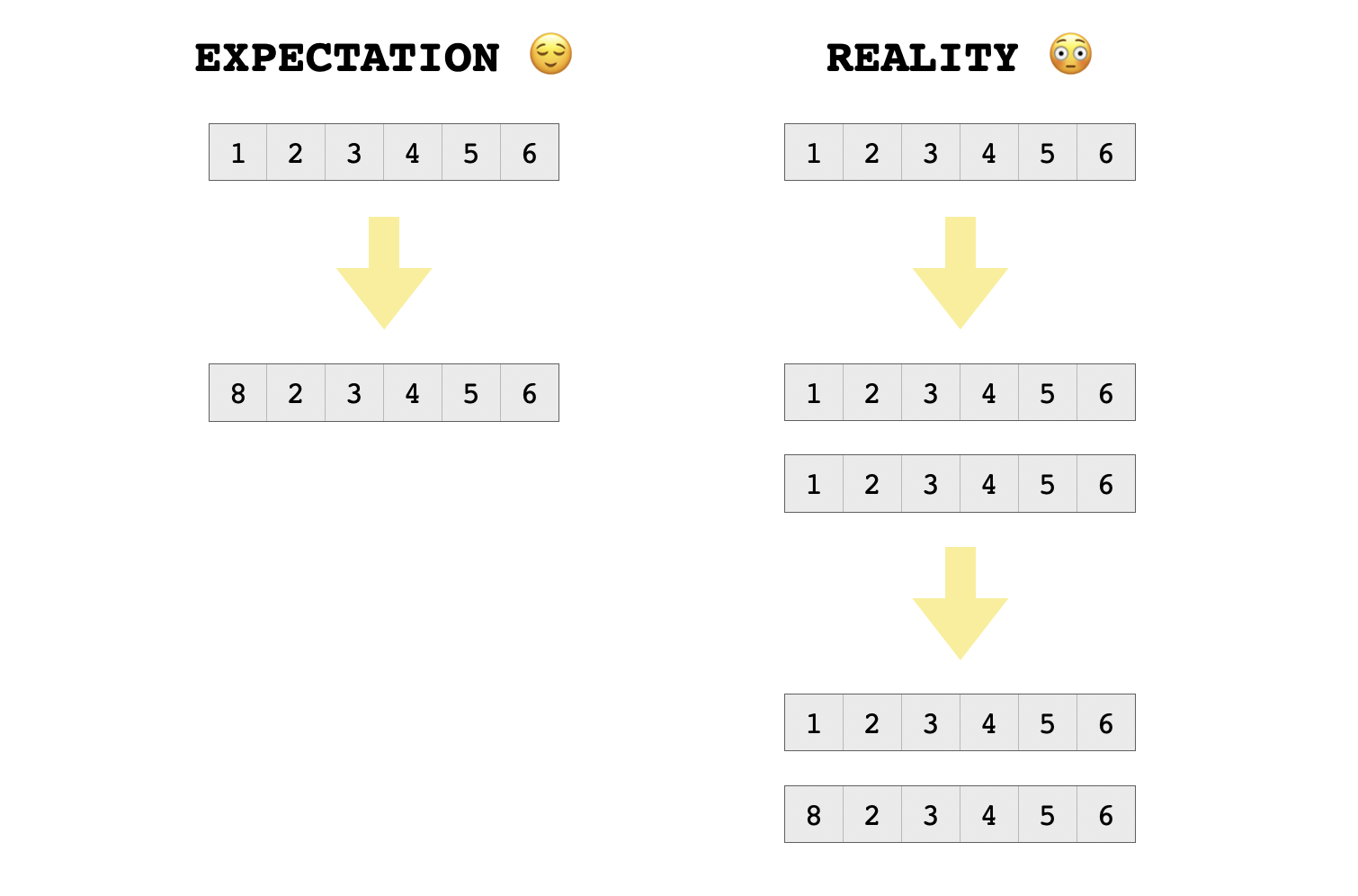
Notice that to the user, this is mostly indistinguishable from copy-on-assignment. A naive R user (such as myself) might have assumed that the vector was copied as soon as we ran y <- x, and there would be nothing in the program’s behavior to contradict this notion - at least, not for simple cases. If you test out the following sequence of commands:
> x <- (1:1e7)^2
> y <- x
> x[1] <- 2
If the language were copy-on-assignment, the first and second commands might cause a noticeable delay, because those would be the commands causing a large chunk of memory to be allocated for a new vector. Instead, if you run these commands in R, you will probably notice a slight lag after the first and third commands, since a second vector does not actually get allocated until mutation is performed. Something like this might tip off an ignorant (but astute) user that copy-on-write is being used.
Now let’s play with lists a little. We can create an inspect a list of vectors like this:
> ls <- list(c(1,2,3), c(4,5,6))
> .Internal(inspect(ls))
@563364786668 19 VECSXP g0c2 [REF(1)] (len=2, tl=0)
  @5633657b8da8 14 REALSXP g0c3 [REF(1)] (len=3, tl=0) 1,2,3
  @5633657b8d58 14 REALSXP g0c3 [REF(1)] (len=3, tl=0) 4,5,6
As before, I can modify the vectors in-place without entirely new vectors being allocated, since their reference counts are equal to one and they aren’t shared:
> ls[[1]][1] <- 7
> .Internal(inspect(ls))
@563364786668 19 VECSXP g0c2 [REF(1)] (len=2, tl=0)
  @5633657b8da8 14 REALSXP g0c3 [REF(1)] (len=3, tl=0) 7,2,3
  @5633657b8d58 14 REALSXP g0c3 [REF(1)] (len=3, tl=0) 4,5,6
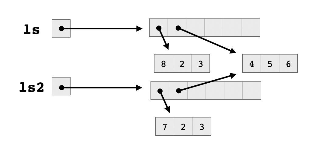
What happens when I assign the list ls to another list ls2 is interesting, though. Check it out:
> ls2 <- ls
> .Internal(inspect(ls))
@563364786668 19 VECSXP g0c2 [REF(2)] (len=2, tl=0)
  @5633657b8da8 14 REALSXP g0c3 [REF(1)] (len=3, tl=0) 7,2,3
  @5633657b8d58 14 REALSXP g0c3 [REF(1)] (len=3, tl=0) 4,5,6
> .Internal(inspect(ls2))
@563364786668 19 VECSXP g0c2 [REF(2)] (len=2, tl=0)
  @5633657b8da8 14 REALSXP g0c3 [REF(1)] (len=3, tl=0) 7,2,3
  @5633657b8d58 14 REALSXP g0c3 [REF(1)] (len=3, tl=0) 4,5,6
The reference count for the VECSXP increased to two, but the reference count for both of the REALSXP vectors stayed at one. Remember how a list in R consists of a block of pointers stored contiguously, which point to structures located elsewhere in memory that constitute the elements of the list? The above output tells us that ls and ls2 share their block of pointers, which means that there is still only one pointer to each of the vectors constituting the elements of these lists.
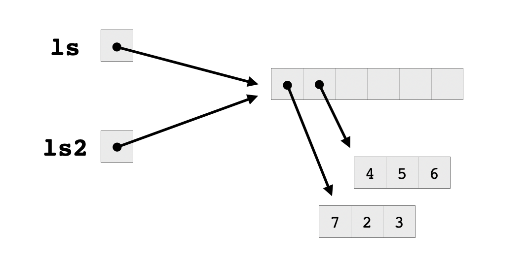
Even though the reference counter of each of the two vectors is set to one, they will still need to be copied upon modification, since they are shared between the two lists. Otherwise, assigning to an element of one list would also affect the elements of the other list, which is exactly the kind of weird side-effect that copy-on-write is meant to protect against. So here’s what happens when we try assigning to an element of one of these vectors:
> ls[[1]][1] = 8
> .Internal(inspect(ls))
@56336473b5f8 19 VECSXP g0c2 [REF(1)] (len=2, tl=0)
  @5633657b8ad8 14 REALSXP g0c3 [REF(1)] (len=3, tl=0) 8,2,3
  @5633657b8d58 14 REALSXP g0c3 [REF(2)] (len=3, tl=0) 4,5,6
> .Internal(inspect(ls2))
@563364786668 19 VECSXP g0c2 [REF(1)] (len=2, tl=0)
  @5633657b8da8 14 REALSXP g0c3 [REF(1)] (len=3, tl=0) 7,2,3
  @5633657b8d58 14 REALSXP g0c3 [REF(2)] (len=3, tl=0) 4,5,6
Note that the two lists still share the second vector, which has not yet been modified. However, they no longer share a block of pointers, since their first elements point to two different vectors. Now there are two pointer blocks, each with a reference count equal to one, and the second vector has a reference count equal to two because it’s pointed to by two different lists.
Finally, let’s inspect a data frame.
> df <- data.frame(a=c(1,2,3), b=c(4,5,6))
> .Internal(inspect(df))
@5633642ee988 19 VECSXP g0c2 [OBJ,REF(4),ATT] (len=2, tl=0)
  @563365901c28 14 REALSXP g0c3 [REF(5)] (len=3, tl=0) 1,2,3
  @563365901bd8 14 REALSXP g0c3 [REF(5)] (len=3, tl=0) 4,5,6
ATTRIB:
  @563365926da8 02 LISTSXP g0c0 [REF(1)]
    TAG: @56336398bee0 01 SYMSXP g0c0 [MARK,REF(5733),LCK,gp=0x4000] "names" (has value)
    @5633642eeb88 16 STRSXP g0c2 [REF(65535)] (len=2, tl=0)
      @563363c6f4b8 09 CHARSXP g0c1 [MARK,REF(21),gp=0x61] [ASCII] [cached] "a"
      @563363f845d0 09 CHARSXP g0c1 [MARK,REF(26),gp=0x61] [ASCII] [cached] "b"
    TAG: @56336398c420 01 SYMSXP g0c0 [MARK,REF(13689),LCK,gp=0x4000] "class" (has value)
    @5633657e22f8 16 STRSXP g0c1 [REF(65535)] (len=1, tl=0)
      @563363a36018 09 CHARSXP g0c2 [MARK,REF(278),gp=0x61,ATT] [ASCII] [cached] "data.frame"
    TAG: @56336398bcb0 01 SYMSXP g0c0 [MARK,REF(65535),LCK,gp=0x4000] "row.names" (has value)
    @563365919b48 13 INTSXP g0c1 [REF(65535)] (len=2, tl=0) -2147483648,-3
You can ignore what comes after ATTRIB - this indicates where metadata such as the column names are stored. The important part is at the beginning, where we can see that both of the column vectors we have used to initialize this dataframe already have reference count equal to five. This means that there is no "grace period" during which we can mutate these vectors without the penalty of copying them in their entirety. As soon as we attempt an assignment to any column, that entire column will be replaced. And if we try assigning to a whole row, which has an entry in each column, the whole dataframe will be copied. Yikes.
I’m still not sure where these four additional mystery references come from, but a careful reading of the data.frame source code may reveal the answer.
Herein lies the real problem with my earlier solution. In theory, the algorithm that I described was fine, but I wasn’t aware that it was so important in practice to watch out for unnecessary copying of data structures. In my original implementation, I started with a preallocated dataframe of the appropriate size filled with the placeholder value NA and iteratively filled it by replacing the placeholder data with aggregate data, one group of flows at a time. Because dataframe columns can inexplicably have a high reference count, many of these updates probably resulted in entire columns being copied. And these columns were quite long, since there are about 40,000 different flow groups in the dataset.
How to prevent this? The obvious way is to just not use dataframes, at least not while doing aggregation. Rather than allocating a huge dataframe and loading our partial results into its columns bit by bit, we can just store our partial results in a plain list. Then, when we’re all done with our computations, we can use a function like cbind to efficiently glue the partial results together into a dataframe all at once.
In the end, here’s the implementation that has worked the best for me. It’s heavily inspired by the source code of the standard library function aggregate, though the below actually works faster for me than a solution based on aggregate.
efficient_flow_agg <- function(dat, col_grouping, gpcol_name="GroupMembership") {
    groups <- as.factor(dat[[gpcol_name]]);
    out_list <- list();
    for (g in 1:(length(col_grouping))) {
        gp <- col_grouping[[g]];
        which_cols <- gp[[1]];
        preproc <- gp[[2]];
        postproc <- gp[[3]];
        aggfun <- gp[[4]];
        sel_dat <- preproc(dat[which_cols]);
        gp_list <- lapply(sel_dat, function(cvec) {
            unlist(lapply(split(cvec, groups), aggfun));
        });
        out_list <- c(out_list, postproc(gp_list));
    }
    as.data.frame(do.call(cbind, out_list))
}
The inputs are dat, the dataframe to be processed, and col_grouping, a list of records defining the groups of codependent columns, each of which takes the following form:
list(
   [VECTOR OF COLUMN NAMES],
   [TRANSFORMATION ON STATISTICS],
   [INVERSE TRANSFORMATION ON STATISTICS],
   [AGGREGATION FUNCTION TO BE FOLDED]
)
For instance, for a triple of columns measuring duration and average packet rate, the corresponding col_grouping record might look like this:
list(
   c("duration", "avg_packet_rate"),
   function(df) {
       data.frame(
           duration = df$duration,
           tot_packets = df$duration * df$avg_packet_rate
       )
   },
   function(df) {
       data.frame(
           duration = df$duration,
           avg_packet_rate = df$tot_packets / df$duration
       )
   },
   sum
)
The next time I write some R code that takes unacceptably long to run, my first move will be to look for steps in my code that might have triggered unnecessary copying.