Skip to page content Home     Posts     CV     Contact     People

Multidimensional integrals

2018 March 30

Calculate the following integrals: $$\int_{-\infty}^\infty e^{-x^2}dx$$ $$\int_0^\infty e^{-x}\text{erf}(\sqrt x)dx$$ $$\int_0^\infty e^{-z}\text{erf}^2(\sqrt z)dz$$

Before diving into some properties and tricks surrounding each type of integral, I would first like to explore the properties of integrals (single, double, and triple) as well as their conversions between different coordinate systems in order to help the reader build an intuition about them - an intuition that will be valuable for the problems at the end, and in later posts.

NOTE: At the very beginning, I will explain and describe each type of integral, and later in the post, I will provide examples. Feel free to hop back and forth between the descriptions and examples if you feel like you need to see a more concrete example of each integral in order to understand them better.

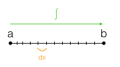
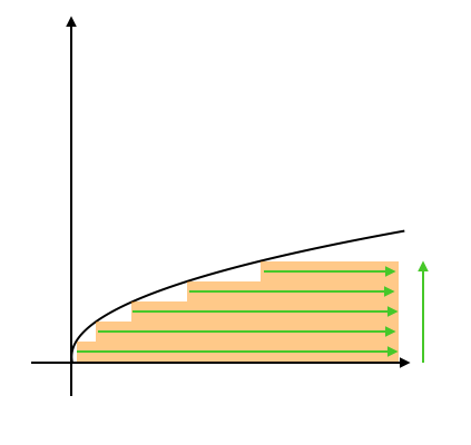
Consider a plain, simple integral in the form $$\int_a^b f(x)dx$$ From the very definition of an integral, it is obtained by cutting up the interval of integration into infinitely many infinitesimally small subintervals and summing up the values of the function on each of those intervals. Simply summing infinitely many values of a function would result in a non-finite number, so the value of the function on each interval is "weighted" by multiplying it by the infinitesimal length of the interval, or $dx$. The infinite number of intervals and the infinitesimal length of each balance each other out, resulting in a finite value.

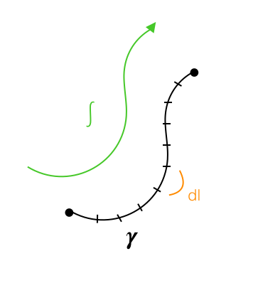
The next most complicated type of integral is the line integral, which integrates over a continuous path in the cartesian coordinate plane rather than a straight line segment on the real line. When one takes a line integral between two points in the coordinate plane, it isn't enough to simply specify which two points the integral goes between - one must also specify the path across which one integrates. If $\gamma$ is a path in the coordinate plane, then the line integral would be written as $$\int_\gamma f(x,y)dl$$ Again, we divide up the path over which the integral is taken, but it isn't an interval anymore, so it has to be divided up differently. We cut the path up into infinitely many infinitesimal pieces. But because we are no longer working on the real line, we can't use $dx$ as the length of each path, because the path transcends the $x$-dimension and moves in the $y$-dimension as well. Instead, we use $dl$, which is the infinitesimal length of each mini-path.

One might wonder how exactly to evaluate such an integral with respect to $l$ when $l$ appears nowhere in the integrand itself. One might try to do so by calculating $dl$ in terms of $dx$ and $dy$.

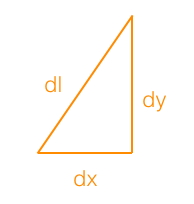
However, this does not lead to a very helpful result. By using the pythagorean theorem, we have simply $$(dl)^2=(dx)^2+(dy)^2$$ This may seem fallacious, since our path is not necessarily a straight line, and the pythagorean theorem applies only to triangles with straight sides. However, because these paths are infinitesimally small, they have no choice but to look more and more like line segments as they grow smaller and smaller.

Unfortunately, this does not help us much, since $$\int_\gamma f(x,y)\sqrt{(dx)^2+(dy)^2}$$ does not make much sense. However, the problem can be solved by parametrizing the integral. Let $x$ and $y$ be functions of $t$ such that the point $(x,y)$ moves from one endpoint of the path to the other as $t$ goes from $0$ to $1$. Then notice that our integral is equal to $$\int_\gamma f(x,y)\sqrt{\bigg(\frac{dx}{dt}\bigg)^2+\bigg(\frac{dy}{dt}\bigg)^2}dt$$ or, since the path is travelled completely from $t=0$ to $t=1$, and $t$ has become our new variable of integration, $$\int_0^1 f(x,y)\sqrt{\bigg(\frac{dx}{dt}\bigg)^2+\bigg(\frac{dy}{dt}\bigg)^2}dt$$ Notice, interestingly, that if $f(x,y)=1$, this integral computes the length of the path over which it is taken.

So far, we have been using cartesian coordinates, but recall that there is one other prominent two-dimensional coordinate system: polar coordinates. Suppose our function $f$ is instead a function of $r$ and $\theta$, and a conversion to cartesian coordinates would be unnecessarily messy. Then we would consider the line integral $$\int_\gamma f(r,\theta)dl$$ Conveniently, we can construct another shape that resembles a triangle as the lengths become infinitesimal, allowing us to treat it as such. Since the length of an $d\theta$-radian arc of a circle with radius $r$ is given by $rd\theta$, we can construct the following diagram:

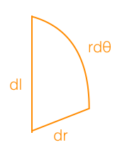
This allows us to say that $$(dl)^2=r^2(d\theta)^2+(dr)^2$$ If we proceed as before using parametrization, we will end up with the following final result: $$\int_0^1 f(r,\theta)\sqrt{r^2\bigg(\frac{d\theta}{dt}\bigg)^2+\bigg(\frac{dr}{dt}\bigg)^2}dt$$

Now I shall move on to the next type of integral, which is a double integral. The double integral is taken over a two-dimensional region in the coordinate plane rather than a one-dimensional path. Instead of dividing it up into segments as we did with line integrals, in order to weight the function values, we must divide the area into patches and multiply the function value on each patch by the area of the patch. Thus, for an integral over a region $R$, we would have $$\iint_R f(x,y)dA$$ where $dA$ is an infinitesimally small patch of area. However, this is of no use to us as it is, since the integral is taken with respect to area $A$, not $x$ or $y$. We can compute $dA$ in terms of $dx$ and $dy$, however, by cutting up the region of integration using horizontal and vertical lines:

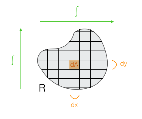
Because a small rectangular patch $dA$ has side lengths $dx$ and $dy$, we can say that $$dA=dxdy$$ It may seem worrying that the region of integration has some non-rectangular patches cut off on the sides, but as our $dx$ and $dy$ become infinitesimal, these rough patches become so tiny that we can ignore them, while the majority of the region is tiled by rectangles. Thus, the integral over a region is $$\iint_R f(x,y)dxdy$$

Again, sometimes it is more convenient to use polar coordinates. If this is the case, then one would have to divide up the region into equiangular and equiradial lines as shown below:

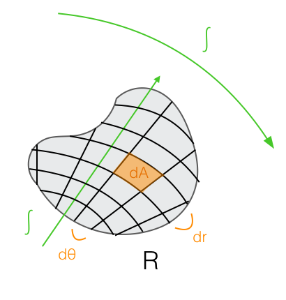
Each of these tiny pieces has the following measurements:

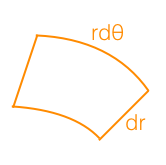
Now, these pieces are parts of circle sectors, but as we make them smaller and smaller, they will begin to look like rectangles with side lengths $rd\theta$ and $dr$, so we will just treat them like rectangles and say that $dA=rdrd\theta$. Thus, we have that the integral of the function $f(r,\theta)$ over the region $R$ is given by $$\iint_R f(r,\theta)r drd\theta$$

Of course, just like normal integrals along line segments on the real line can be extended to line integrals not confined to the real line, integrals over regions can be extended to integrals over two-dimensional surfaces that curve and protrude into three dimensions. They can be calculated similarly, so I will skip them.

Instead, I will talk about three-dimensional integrals, which use three different prominent coordinate systems: cartesian, cylindrical, and spherical. A triple integral would typically be taken over a three-dimensional volume, and because of this, the differential area $dA$ is replaced by $dV$, the differential volume. In cartesian coordinates, the differential volume is easy to calculate by splitting a volume up into tiny rectangular prisms:

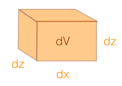
This tells us that $dV=dxdydz$.

Cylindrical coordinates are basically a projection of polar coordinates into the third dimension by adding height to the polar coordinate plane. In cylindrical coordinates, a point is determined by an angle $\theta$, a radius $r$ from the $z$-axis, and a height $z$. We found $dA$ for polar coordinates by cutting the region up into circle sector pieces, but when a height is added in cylindrical coordinates, we just added height to each circle sector piece to make it a prism.

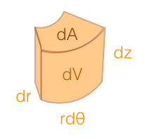
The volume of this prism will just be its base area $dA$ times its new height $dz$, so for cylindrical coordinates, $dV=rdrd\theta dz$.

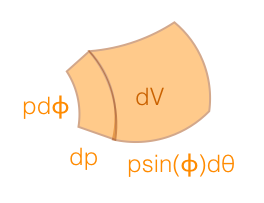
Spherical coordinates are only slightly trickier. In spherical coordinates, a point is determined by a radius $\rho$ from the origin, an angle $\theta$ measured the same way as in cylindrical coordinates, and an angle $\phi$ measured down from the $z$-axis to the point. This way, a region can be cut up into mini-solids that approach rectangular prisms as they grow smaller:

The complexity of $dV$ in spherical coordinates surpasses my diagram-making skills, so I'll have to bring in a diagram from elsewhere:

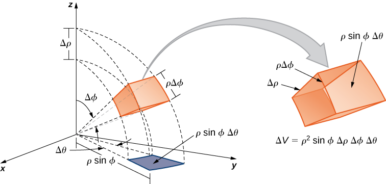
This tells us that $dV=\rho^2\sin\phi d\rho d\phi d\theta$. This one can be hard to visualize, but there are plenty of awesome diagrams online that illustrate it very nicely.

This can be extended even into three dimensions and even further, but that is for another post. For now, I'll provide examples of the types of integrals that I have described so far, and a few applications. I will skip the normal one-dimensional integral, which I'm sure the reader is familiar with, and will begin immediately with an example of a line integral.

Of course, the obvious example of a line integral is the integral of $1$ over a curve to find the arclength of the curve. Instead, I would like to use an example from physics.

In physics, if a particle is dragged through a force field, the work done on it by the force field is given by $$W=\int_\gamma \overrightarrow{F}\cdot \overrightarrow{ds}$$ where $\gamma$ is the path that the particle is dragged across, $\overrightarrow{F}$ is the force vector of the field at any point, $\cdot$ is a dot product, and $\overrightarrow{ds}$ is the displacement of the particle over a miniscule amount of time. The work done by the person dragging it is given by $-W$.

Consider now the force field created by gravity (on a small scale) with a force of $g$ directed downwards. Suppose we have a particle with a mass of $m$ and we move it along the curve $y=x^2$ starting at $(0,0)$ and ending at $(2,4)$. Then we have the integral $$W=\int_\gamma \langle 0, -mg \rangle \cdot \langle dx,dy \rangle$$ or, by parametrizing with $x=t$ and $y=t^2$ from $t=0$ to $2$, $$\begin{align} W &=\int_\gamma \langle 0, -mg \rangle \cdot \langle dx/dt,dy/dt \rangle dt\\ &=\int_0^2 \langle 0, -mg \rangle \cdot \langle 1,2t \rangle dt\\ &=\int_0^2 -2mgt dt\\ &=-4mg \end{align}$$

It makes sense that $W$ is negative, since the particle moves against the forces of the gravitational force field. Interestingly, in the field of physics, a force field $\overrightarrow{F} (x,y)$ is called conservative if the work done by it on a particle as the particle moves between two points is the same regardless of the path taken by the particle.

An application of a double integral over a region is the calculation of volume. If a solid's base is a region $R$ and its height above a point $(x,y)$ in the region is given by $h(x,y)$, then its volume is given by $$\iint_R h(x,y) dA$$ Intuitively, this can be shown by slicing the solid up into infinitely many infinitesimally small rectangular prisms using cuts parallel to the $x$ and $y$ axes. Each prism would have dimensions $dx$, $dy$, and $h(x,y)$, making the volume of the prism above the point $(x,y)$ be given by $h(x,y)dxdy$. For example, the volume underneath the surface given by $z=1+x+\sin(y)$ above the square region with vertices $(0,0)$, $(1,0)$,$(0,\pi)$, and $(1,\pi)$ is given by

$$\begin{align} \iint_R (1+x+\sin(y))dxdy &=\int_0^\pi \int_0^1 (1+x+\sin(y))dxdy\\ &=\int_0^\pi \bigg[x+x^2/2+x\sin(y)\bigg]_0^1dy\\ &=\int_0^\pi \bigg(\frac{3}{2} +\sin(y)\bigg)dy\\ &=\bigg[\frac{3}{2}y-\cos(y)\bigg]_0^\pi\\ &=\frac{3\pi}{2}-2\\ \end{align}$$

As stated earlier, sometimes it is helpful to use polar coordinates. Consider the solid below the surface $z=1-x^2-y^2$ (which, by the way, is a paraboloid) and above the unit circle in the $x$- $y$ plane. If we tried using an integral in cartesian coordinates, we would get $$\int_{-1}^1 \int_{-\sqrt{1-y^2}}^{\sqrt{1-y^2}}(1-x^2-y^2)dxdy$$ ...and that's no fun at all. Radicals are yucky to integrate. But if we convert it to polar coordinates, we get something much nicer. We can replace $x^2+y^2$ with $r^2$ and $dxdy$ with $rdrd\theta$, and the bounds change to constants (since the radius of a circle is constant all the way around), giving us $$\int_0^{2\pi} \int_0^1 r(1-r^2)drd\theta=\frac{\pi}{2}$$

Now I will demonstrate a few tricks using the concepts that I've already described. First, I will rederive the Gaussian Integral using these tricks, whose value I first derived in this post: $$\int_{-\infty}^\infty e^{-x^2}dx$$ This is equal to $$\sqrt{\bigg(\int_{-\infty}^\infty e^{-x^2}dx\bigg)^2}$$ or $$\sqrt{\bigg(\int_{-\infty}^\infty e^{-x^2}dx\bigg) \bigg(\int_{-\infty}^\infty e^{-y^2}dy\bigg)}$$ Now, because of the linearity of integrals, the product of the integrals of two functions is equal to the double integral of their product. This gives us $$\sqrt{\int_{-\infty}^\infty \int_{-\infty}^\infty e^{-x^2-y^2}dxdy }$$ or, since the entire real plane is covered as both $x$ and $y$ go from negative infinity to infinity, and since $dA=dxdy$, $$\sqrt{\iint_{\mathbb R} e^{-x^2-y^2}dA }$$ This is where I shall apply some of the properties of double integrals over regions that I described before. I showed that $dA$ is equal to $dxdy$, but also that it is equal to $rdrd\theta$. Notice also that $-x^2-y^2=-r^2$. Thus, I can convert this double integral in cartesian coordinates to a double integral in polar coordinates. In doing this, I must also change the bounds, since the real plane is covered by a radius stretching from $0$ to $\infty$ and an angle sweeping from $0$ to $2\pi$. Thus, I have $$\sqrt{\int_0^{2\pi}\int_0^\infty re^{-r^2}drd\theta }$$ The integrand now has an elementary antiderivative, so the value can be computed at once: $$\begin{align} \int_{-\infty}^\infty e^{-x^2}dx &= \sqrt{\int_0^{2\pi}\int_0^\infty re^{-r^2}drd\theta }\\ &= \sqrt{2\pi\int_0^\infty re^{-r^2}dr }\\ &= \sqrt{2\pi\bigg[-\frac{e^{-r^2}}{2}\bigg]_0^\infty }\\ &= \sqrt{2\pi\cdot\frac{1}{2} }\\ &= \sqrt\pi\\ \end{align}$$ Giving us the magnificent result $$\bbox[lightgray,5px] { \int_{-\infty}^\infty e^{-x^2}dx=\sqrt\pi }$$

Now consider the related integral $$\int_0^\infty e^{-x}\text{erf}(\sqrt x)dx$$ where "erf" is the error function, defined as $$\text{erf}(x):=\frac{2}{\sqrt\pi}\int_0^x e^{-y^2}dy$$ If we plug this definition into our integral, we obtain $$\frac{2}{\sqrt\pi}\int_0^\infty \int_0^{\sqrt x} e^{-y^2-x}dydx$$ How on earth are we going to integrate this? We don't even know an elementary antiderivative for $e^{-y^2}$!

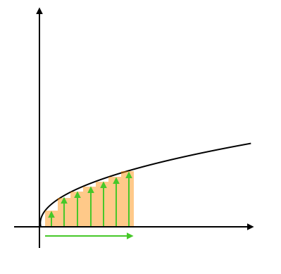
Here's the trick. Notice that the region that we are integrating over is the region in the first quadrant bounded by $y=\sqrt{x}$ and the $x$-axis. Currently, we are integrating first over $y$ and then over $x$, letting our integral fill up little mini-rectangles from top to bottom underneath $y=\sqrt x$, filling up the rectangles one at a time from left to right.

It can be difficult to visualize what the order of integration means, so here's an illustration. The integral, as we currently have it, is done by integrating over the region like this:

...but our integral would yield the same value if we integrated across the region like this instead:

If we did it like this, our integral quickly turns into the famed Gaussian integral, whose value I derived in a . We have: $$\frac{2}{\sqrt\pi}\int_0^\infty \int_{y^2}^{\infty} e^{-y^2-x}dxdy$$ This can be readily evaluated: $$\begin{align} \frac{2}{\sqrt\pi}\int_0^\infty \int_{y^2}^{\infty} e^{-y^2-x}dxdy &= \frac{2}{\sqrt\pi}\int_0^\infty e^{-y^2}[-e^{-x}]_{y^2}^\infty dy\\ &= \frac{2}{\sqrt\pi}\int_0^\infty e^{-y^2}\cdot e^{-y^2}dy\\ &= \frac{2}{\sqrt\pi}\int_0^\infty e^{-2y^2}dy\\ &= \frac{\sqrt 2}{\sqrt\pi}\int_0^\infty e^{-y^2}dy\\ &= \frac{\sqrt 2}{\sqrt\pi}\cdot \frac{\sqrt\pi}{2}\\ &= \frac{1}{\sqrt 2}\\ \end{align}$$

Thus, we have the interesting identity $$\bbox[lightgray,5px] { \int_0^\infty e^{-x}\text{erf}(\sqrt x)dx=\frac{1}{\sqrt 2} }$$

The following similar integral can be evaluated using a similar strategy, but it requires true integral prowess, because the initial volume over which the resulting triple integral is taken is so tricky to visualize, and the change in integration order is difficult to make correctly. Let's begin: $$\int_0^\infty e^{-z}\text{erf}^2(\sqrt z)dz$$ Starting similarly as before, we must expand this into a triple integral this time rather than a double integral, because the error function is squared: $$\frac{4}{\pi}\int_0^\infty \int_0^\sqrt{z} \int_0^\sqrt{z} e^{-x^2-y^2-z}dxdydz$$ As with the previous integral, the trick here is to change the order of integration... however, this time, it is a bit trickier. By looking at the bounds of the integral, we can see that the integral is taken over the infinite solid in the first octant whose cross-section at height $z$ perpendicular to the z-axis is a square with a vertex at $(0,0,z)$ and a side length equal to $\sqrt{z}$. This is also the volume in the first octant above the surface $$z=\max(x^2,y^2)$$ Because we now know the curve above which this volume lies, we may change the order of integration to $$\frac{4}{\pi}\int_0^\infty \int_0^\infty \int_{\max(x^2,y^2)}^\infty e^{-x^2-y^2-z}dzdydx$$ The innermost integral can be easily computed, since we know the antiderivative of $e^{-z}$. We now have the double-integral $$\frac{4}{\pi}\int_0^\infty \int_0^\infty e^{-x^2-y^2-\max(x^2,y^2)}dydx$$ The $\max(x^2,y^2)$ makes things troublesome for us. Notice that this double integral is taken over the entire first quadrant of the $x$-$y$ plane. Let's cut the $x$-$y$ plane in half with the line $y=x$, and integrate separately over each of the resulting regions. This gives us: $$\frac{4}{\pi}\int_0^\infty \int_0^x e^{-x^2-y^2-\max(x^2,y^2)}dydx+\frac{4}{\pi}\int_0^\infty \int_0^y e^{-x^2-y^2-\max(x^2,y^2)}dxdy$$ Notice that below the line $y=x$, or in the region over which the first integral is taken, $y\le x$, meaning that $\max(x^2,y^2)=x^2$. Similarly, in the other region, $\max(x^2,y^2)=y^2$. Thus, we now have $$\frac{4}{\pi}\int_0^\infty \int_0^x e^{-2x^2-y^2}dydx+\frac{4}{\pi}\int_0^\infty \int_0^y e^{-x^2-2y^2}dxdy$$ Notice now that these two integrals are exactly the same, except for the fact that the variables $x$ and $y$ are switched. Because the variable of integration does not matter, we are left with $$\frac{8}{\pi}\int_0^\infty \int_0^x e^{-2x^2-y^2}dydx$$ Now, by substituting $x\to x/\sqrt{2}$, $$\frac{4\sqrt{2}}{\pi}\int_0^\infty \int_0^{x/\sqrt{2}} e^{-x^2-y^2}dydx$$ This integral is taken over the region in the first quadrant under the line $y=x/\sqrt{2}$. We can represent this same region in polar coordinates by letting $r$ go from $0$ to $\infty$ and $\theta$ sweep from $0$ to $\arctan(1/\sqrt{2})=\text{arccot}(\sqrt{2})$. This gives us the integral $$\frac{4\sqrt{2}}{\pi}\int_0^{\text{arccot}(\sqrt 2)} \int_0^{\infty} re^{-r^2}drd\theta$$ which can easily be finished off the same way as the Gaussian Integral to obtain the value $$\frac{2\sqrt{2}\text{arccot}(\sqrt 2)}{\pi}$$ We now have our final answer:

$$\bbox[lightgray,5px] { \int_0^\infty e^{-x}\text{erf}^2(\sqrt x)dx=\frac{2\sqrt{2}\text{arccot}(\sqrt 2)}{\pi} }$$

That slog marks the end of this blog post! As a further challenge, the reader is invited to attempt the integral $$\int_0^\infty e^{-x}\text{erf}^3(\sqrt x)dx$$ which is even more difficult to calculate because it involves a quadruple integral which would require one to visualize a four-dimensional region.