Skip to page content Home     Posts     CV     Contact     People

Iterative Generative Art with Pycairo

Lately I've been playing around with Pycairo, a neat package for Python that is great for creating aesthetically pleasing geometric art. In particular, we can define loops and recursive functions that use Pycairo's drawing capabilities to create deeply nested images that resemble fractals. In this post, I'll share some pieces of generative art that I've created using this technique, the code used to create them, and a few math problems related to the randomnness and nested structure of these images. I'm not going to talk about the basics of Pycairo, but even so, this post should be accessible to anyone who is familiar with Python but not Pycairo. I personally didn't start learning Pycairo by taking a tutorial, but rather by looking at examples of other people's code.

Repeated Polygon Substitution

Fractals are commonly created by starting with a simple geometric object and repeatedly applying some simple transformation to the object. See, for instance, the Koch Snowflake or the Cantor Set. The former can be created by repeatedly adjoining smaller and smaller triangles to the sides of an increasingly complex polygon, and the latter is formed by repeatedly deleting the middle thirds of line segments.

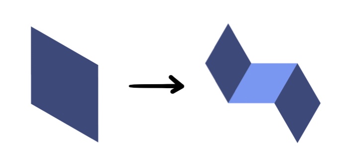
Now I'd like to approximate a fractal that uses a rhombus (with angles of $60^\circ$ and $120^\circ$) as its "starting point" and repeatedly applies the following transformation:

After the image on the left is transformed into the image on the right, each rhombus in the image on the right would be transformed in the same way (accounting for rotation), resulting in the following "second generation" image:

In order to generate image like this, the first thing we need to do is create a function that draws rhombi. Mathematically, we can define the shape and position of a rhombus using four parameters that we will pass to our rhombus-drawing function:

• The coordinates pos = (x0, y0) of one vertex of the rhombus, which we will call the "terminal vertex".
• The side length length of the rhombus (all sides of a rhombus have equal length).
• The angular "tilt" tilt of the rhombus. More specifically, the angle that its "terminal side" makes with the horizontal.
• The angular width ang_width of the rhombus, or the size of the angle at the terminal vertex.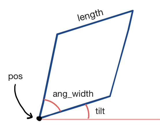

If we want our image to look pretty, we also need to specify what color we want our rhombus to be, so this should be a fifth argument to our rhombus-drawing function. Without further adieu, here's our rhombus-drawing function:

def draw_rhombus(ctx, pos, length, tilt, ang_width, color=[0, 0, 0]):
    x0, y0 = pos
    x1, y1 = x0 + np.cos(tilt) * length, y0 + np.sin(tilt) * length
    x2, y2 = x1 + np.cos(tilt + ang_width) * length, y1 + np.sin(tilt + ang_width) * length
    x3, y3 = x0 + np.cos(tilt + ang_width) * length, y0 + np.sin(tilt + ang_width) * length
    ctx.move_to(x0, y0)
    ctx.line_to(x1, y1)
    ctx.line_to(x2, y2)
    ctx.line_to(x3, y3)
    ctx.line_to(x0, y0)
    ctx.set_source_rgba(*color)
    ctx.fill()

The variable pairs x0, y0 through x3, y3 refer to the coordinates of the vertices of the rhombus, with the first pair being provided as an argument to the function, and the other three being calculated using elementary trig from the angles and side length passed as arguments. You might have noticed that this function has an extra argument called ctx. That's the Cairo Context object, which contains methods like line_to, set_source_rgba, and fill that actually allow us to create images. This will be defined later, just before we actually execute any of our fractal-drawing functions.

Next, we need a function that accepts a rhombus as its argument and returns three rhombi with which it is to be replaced. This time, instead of giving the function distinct arguments for each defining characteristic of the rhombus, we'll represent a rhombus as a list of these parameters, which will be passed to the function as a single argument. More explicitly, each rhombus will be represented by a list of the form [pos, length, tilt, ang_width]. Here's the function:

def replace_rhombus(rhomb):
    pos, length, theta, phi = rhomb
    x0, y0 = pos
    x1, y1 = x0 + np.cos(theta) * length, y0 + np.sin(theta) * length
    x3, y3 = x0 + np.cos(theta + phi) * length, y0 + np.sin(theta + phi) * length
    rhomb1 = [pos, length / np.sqrt(3), theta + phi/2, phi]
    rhomb2 = [(x3, y3), length / np.sqrt(3), theta - 3*phi/2, phi]
    rhomb3 = [(x1, y1), length / np.sqrt(3), theta + phi/2, phi]
    return([rhomb1, rhomb2, rhomb3])

This function is pretty straightforward, and the bulk of its complexity consists of trig calculations. Let's move on to the third and final function.

The last function will generate an array of rhombi that starts out with only one rhombus but grows longer and longer as each rhombus in the array is replaced by three smaller rhombi using the replace_rhombus function. Finally, after repeating this process a specified number of times, it will draw all of the rhombi in the array. Let's take a look:

def generate_fractal(ctx, num_iter):
    rhombi = [[(275, 100), 700, np.pi/6, np.pi/3]]
    for i in range(0, num_iter):
        new_rhombi = []
        for x in rhombi: new_rhombi += replace_rhombus(x)
        rhombi = new_rhombi
    counter = 0
    for r in rhombi:
        counter += 1
        draw_rhombus(ctx, *r, color = COLORS[counter % 2])

In the first line of the function, an array containing our initial rhombus is created. Then a loop is executed that use the replace_rhombus function to replace the previous array of rhombi with a new array in which each old rhombus is replaced by its three "daughter" rhombi. This is carried out num_iter times, and then draw_rhombus is used to draw each rhombus in the array (I've also set it up to alternate between colors while drawing rhombi in the array, just for aesthetic effect). COLORS is an array of RGB colors establishing a color scheme that I've defined at the beginning of the file. As the array of rhombi is looped through, counter is incremented and the color used for each rhombus is determined by counters % 2, which alternates between two values.

Now, to finish up, we need to define the main function and call it to execute the program.

def main():
    surface = cairo.ImageSurface(cairo.FORMAT_ARGB32, 1200, 1200)
    ctx = cairo.Context(surface)
    ctx.set_source_rgb(1, 1, 1)
    ctx.paint()
    generate_fractal(ctx, NUM_ITER)
    surface.write_to_png("gallery/rhomb_fractal_"+str(NUM_ITER)+".png")
if name == "main":
    main()

This function defines the Cairo ImageSurface object, the Context ctx that is passed into all of the functions we call, calls the generate_fractal function, and saves the image to a PNG file. Like COLORS, NUM_ITER is another variable defined elsewhere specifying the "depth" (number of iterations) of the image.

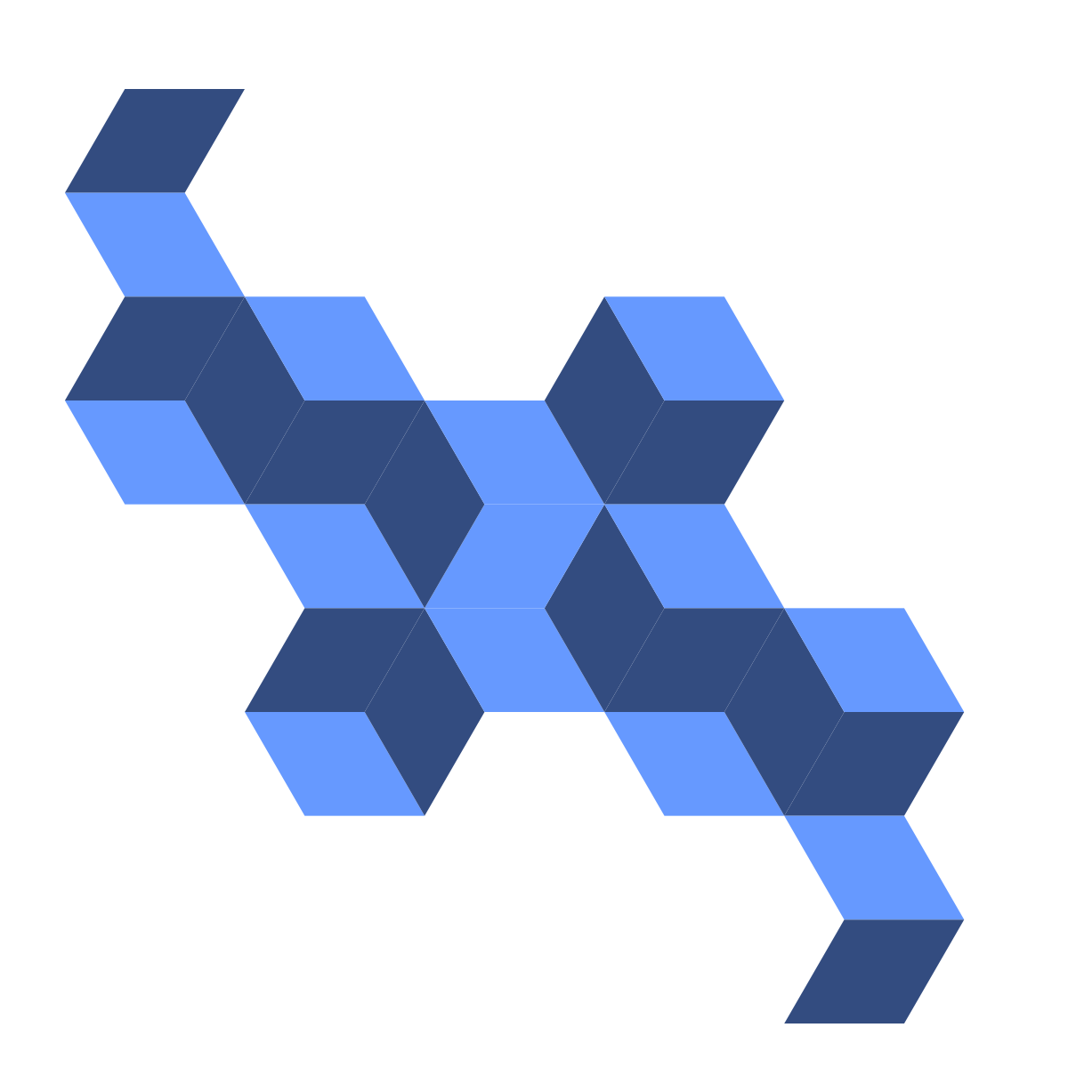
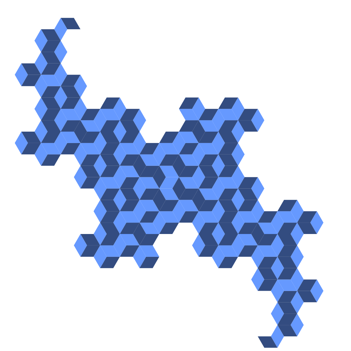
Now that we're finished, let's generate some pretty pictures! You've already seen what the first and second generations look like. Here are generations 3 through 8:

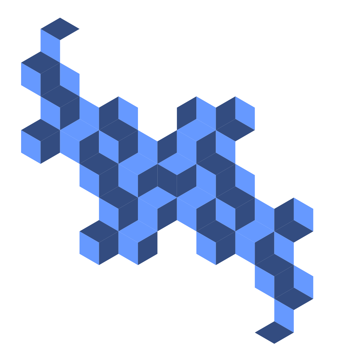
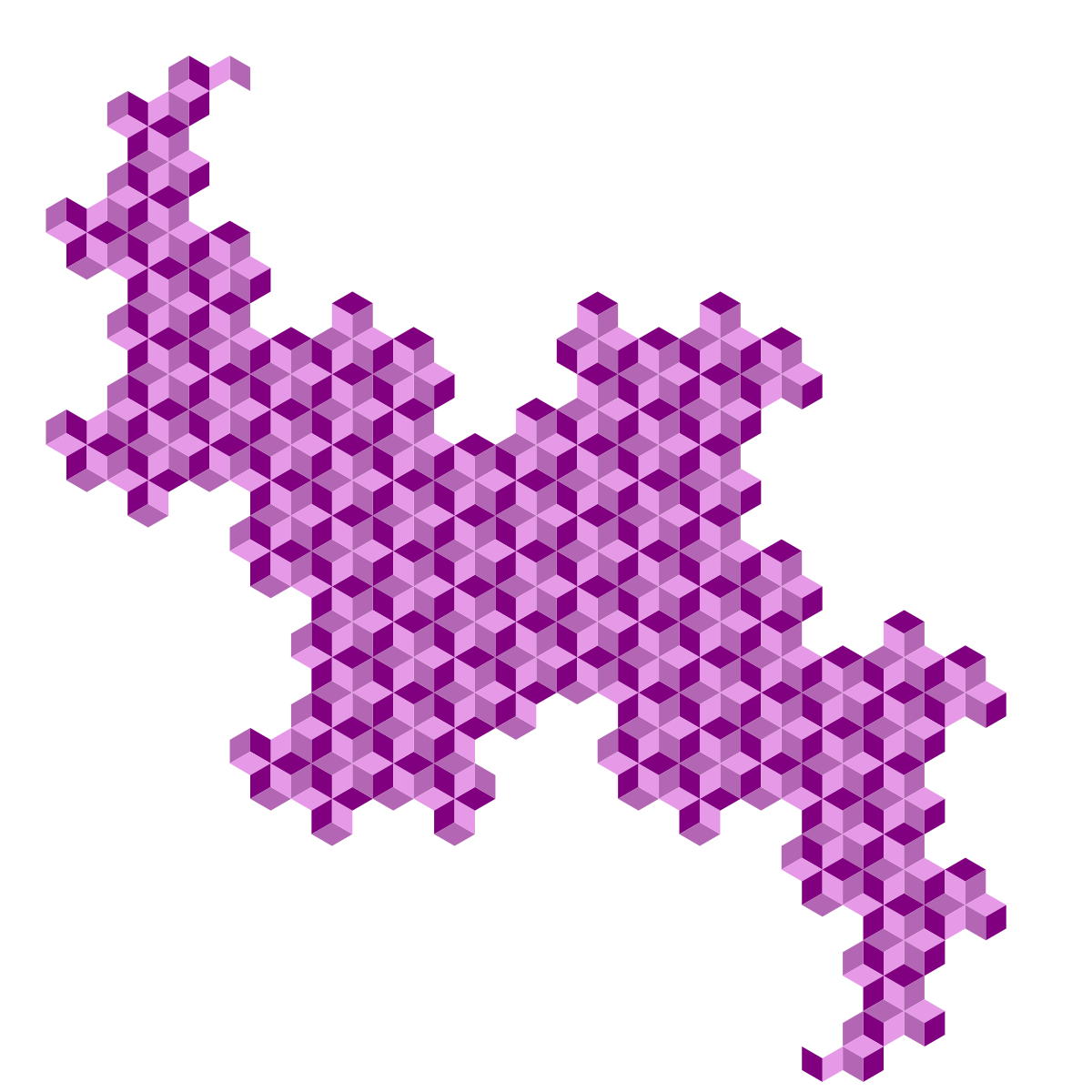
We can also mess around with the color scheme or increase the number of colors used for the rhombi. Here are 3- and 4-color versions of the sixth-generation figure, which I created by altering the color scheme COLORS and replacing COLORS[counter % 2] with COLORS[counter % 3] and COLORS[counter % 4], respectively.

Finally, here are a couple of mathematical questions about the strange object we've just created:

• If the original "zeroth-generation" rhombus has unit area, what is the area of the figure created after $n$ generations? (The answer is simpler than it might seem.)
• If the original rhombus has unit area, what is the perimiter of the figure created after $n$ generations? (This one is trickier.)
• Why does the 3-colored tiling look "more regular" than the 2-colored and 4-colored tilings? Why don't any two rhombi of the same color touch each other in the 3-colored tiling?

Image Shuffling

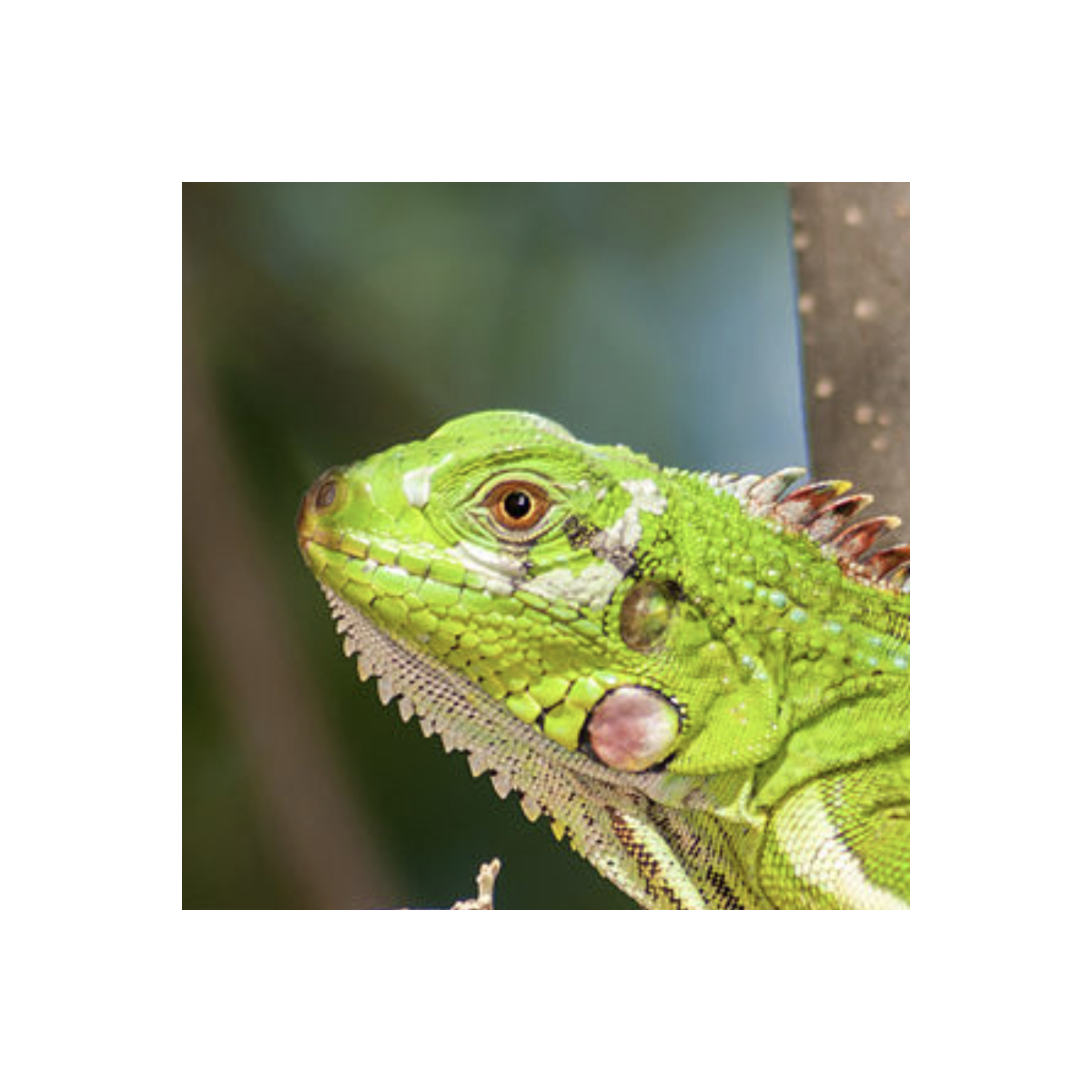
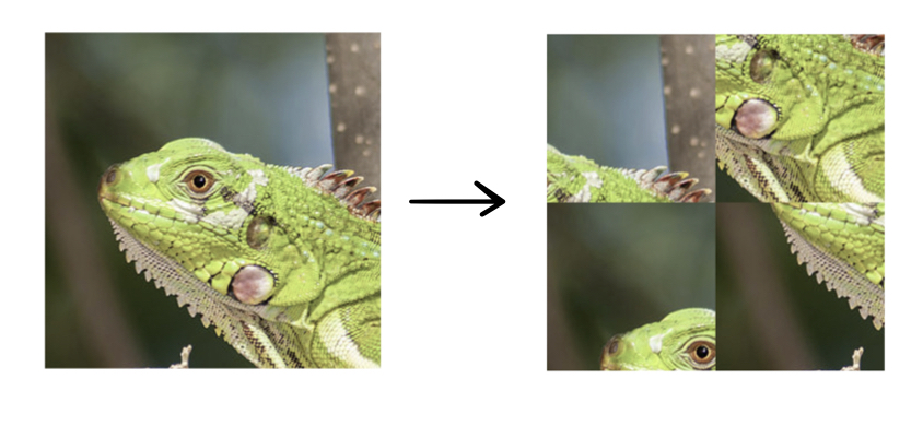
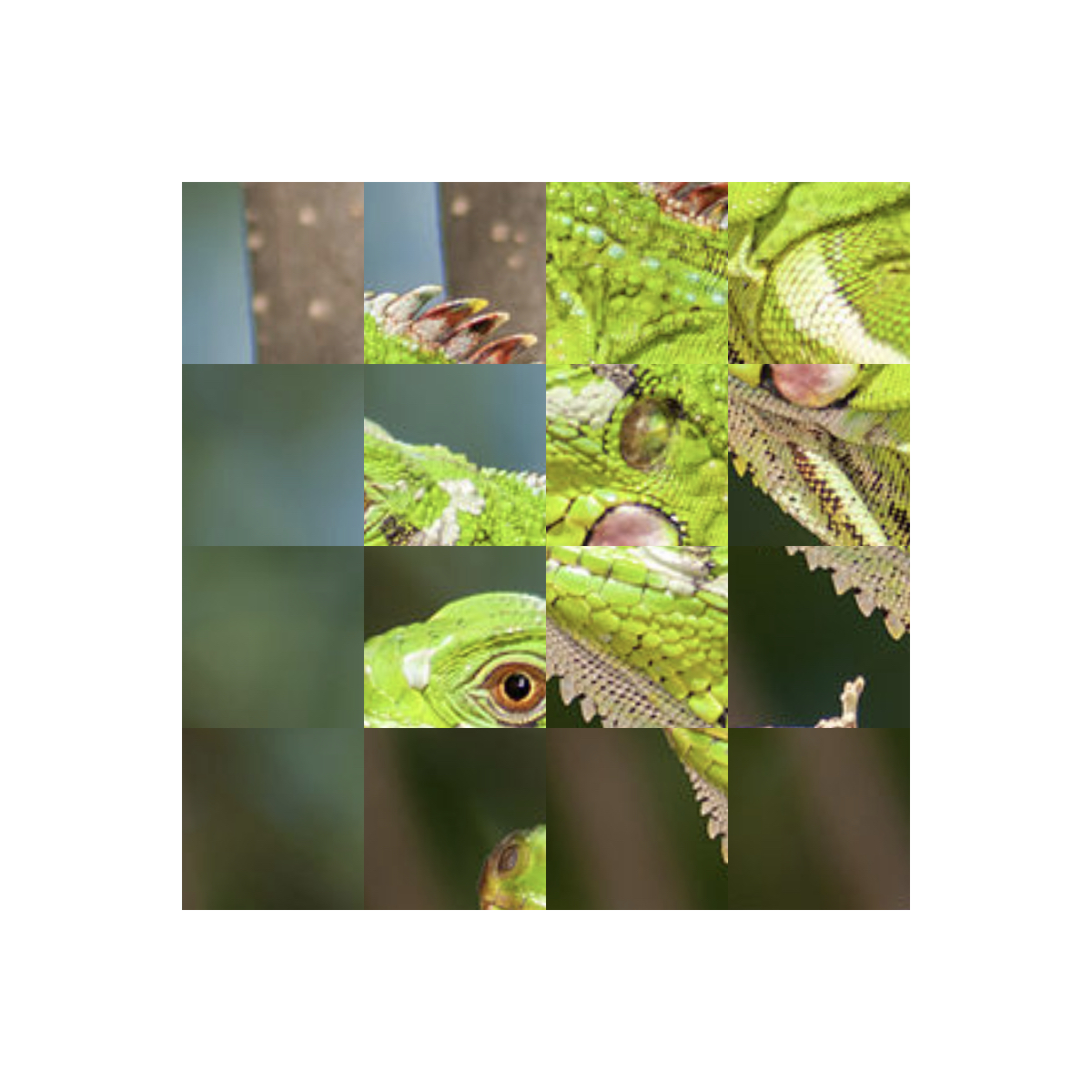
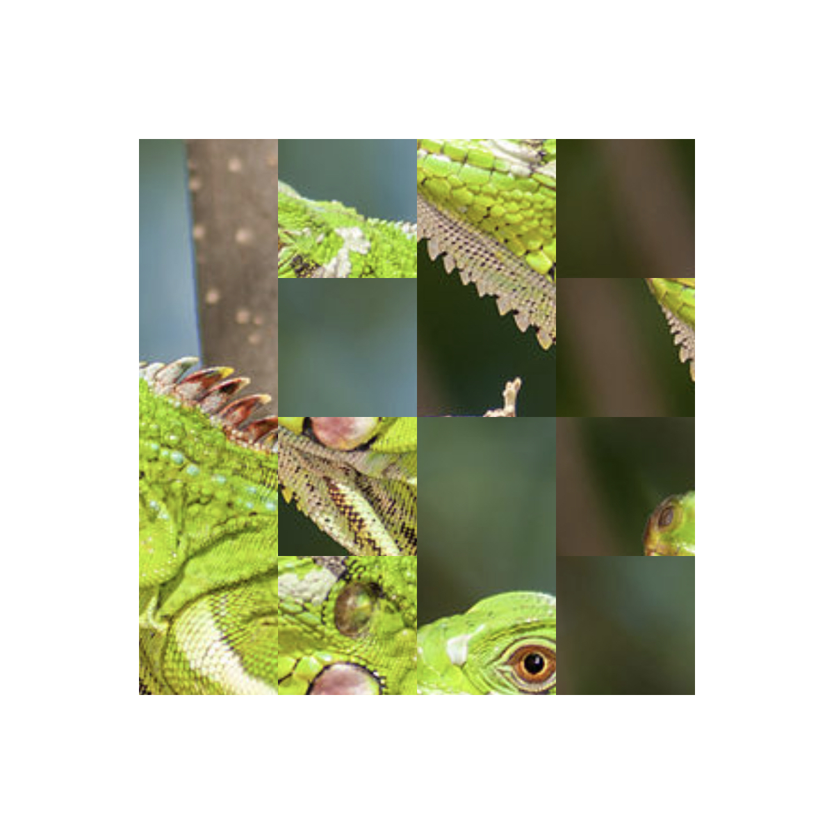
So far we haven't made use of recursion yet, but we will do so in the following example. As before, we will begin with an ordinary, unaltered figure and repeatedly apply a transformation to it. This time, our starting image will be our old friend the iguana, whom we've mutilated once before in an older blog post. Here's the handsome fellow in his natural state:

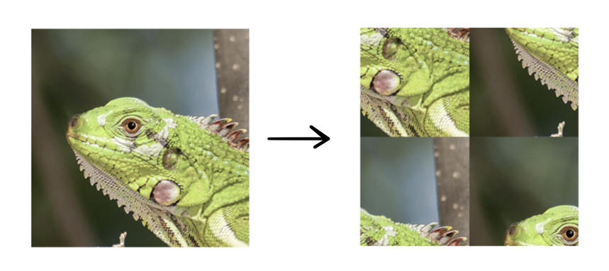
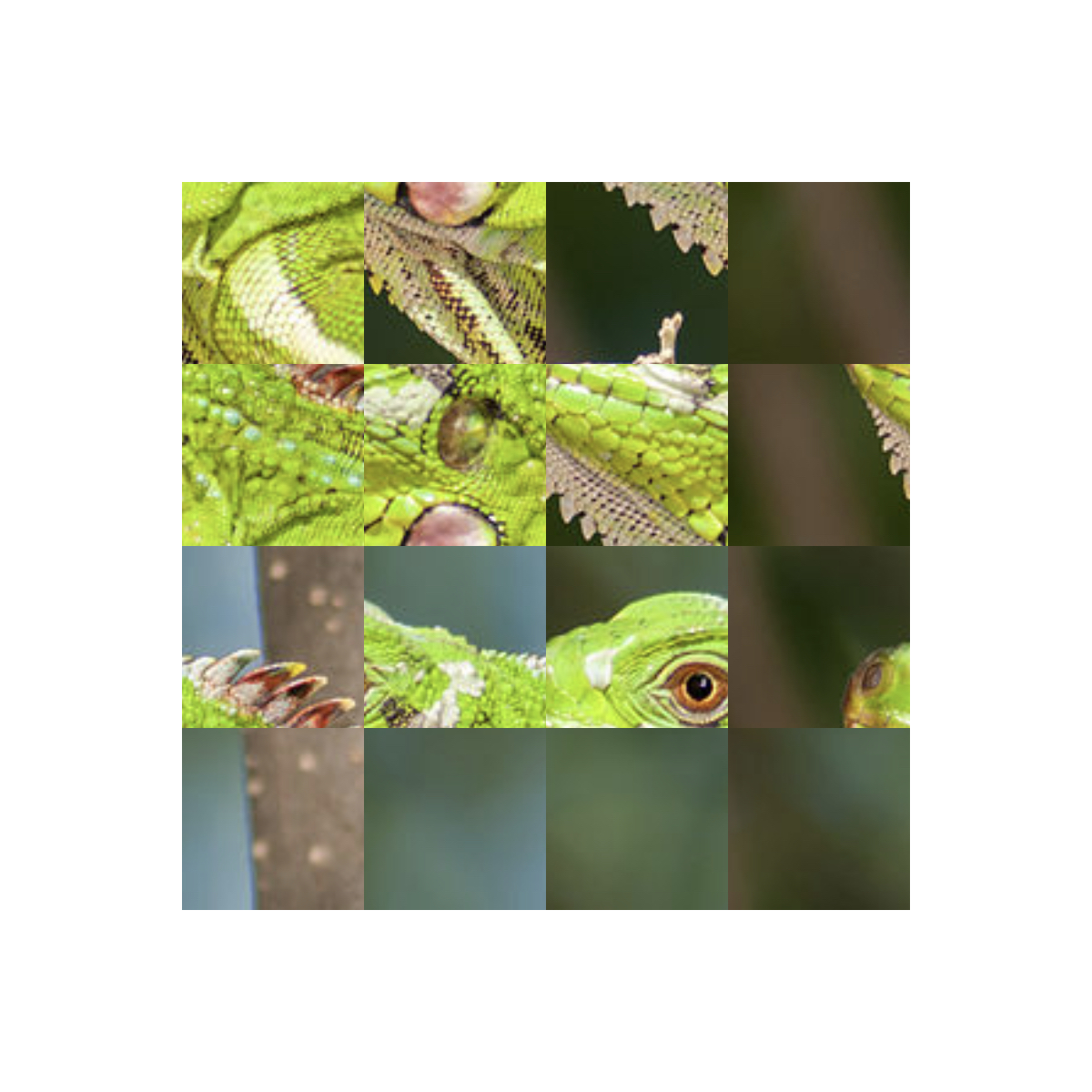
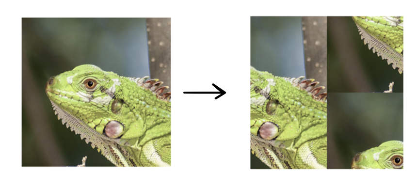
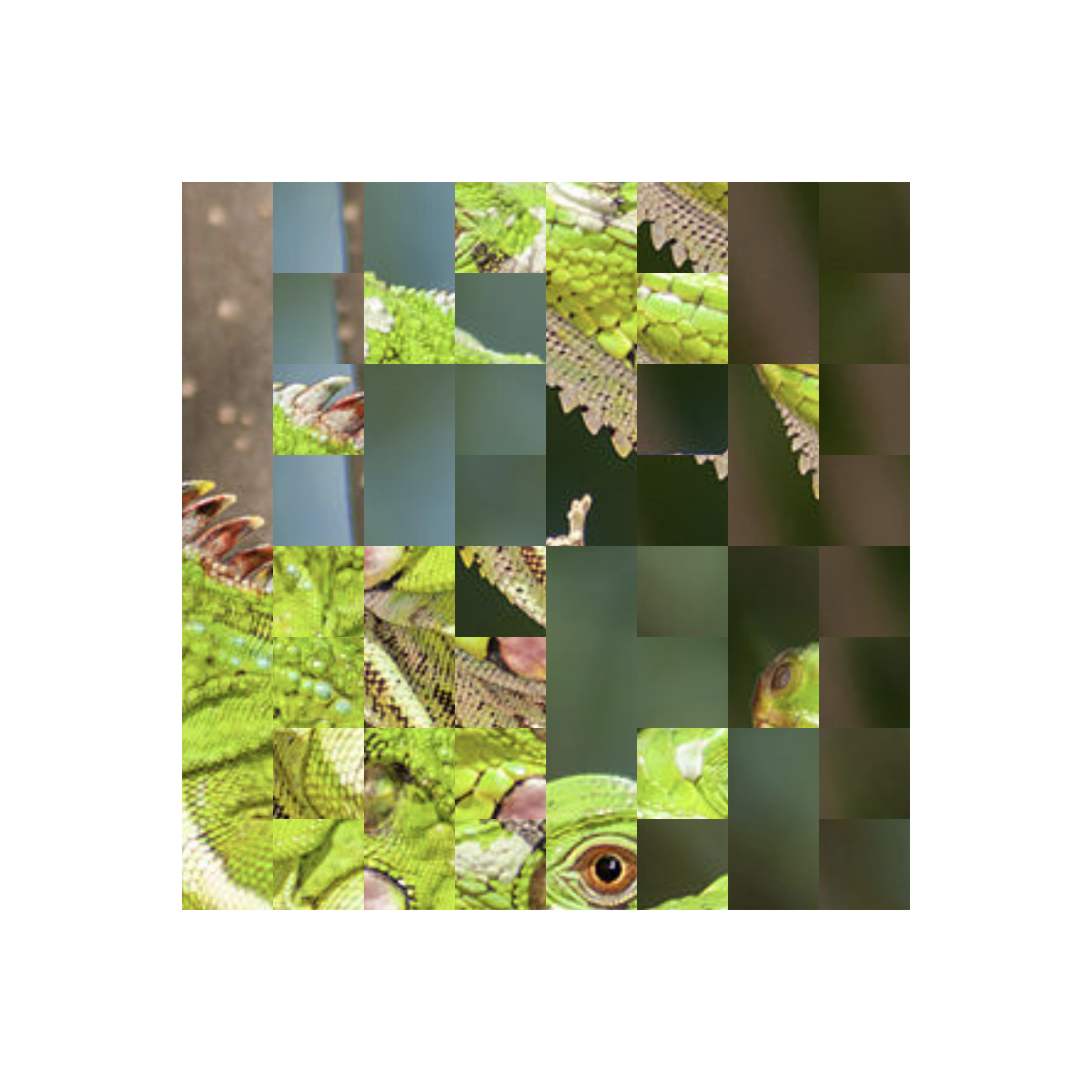
A square image like this can be "shuffled" by cutting it up into quadrants and rearranging the quadrants, say, like this:

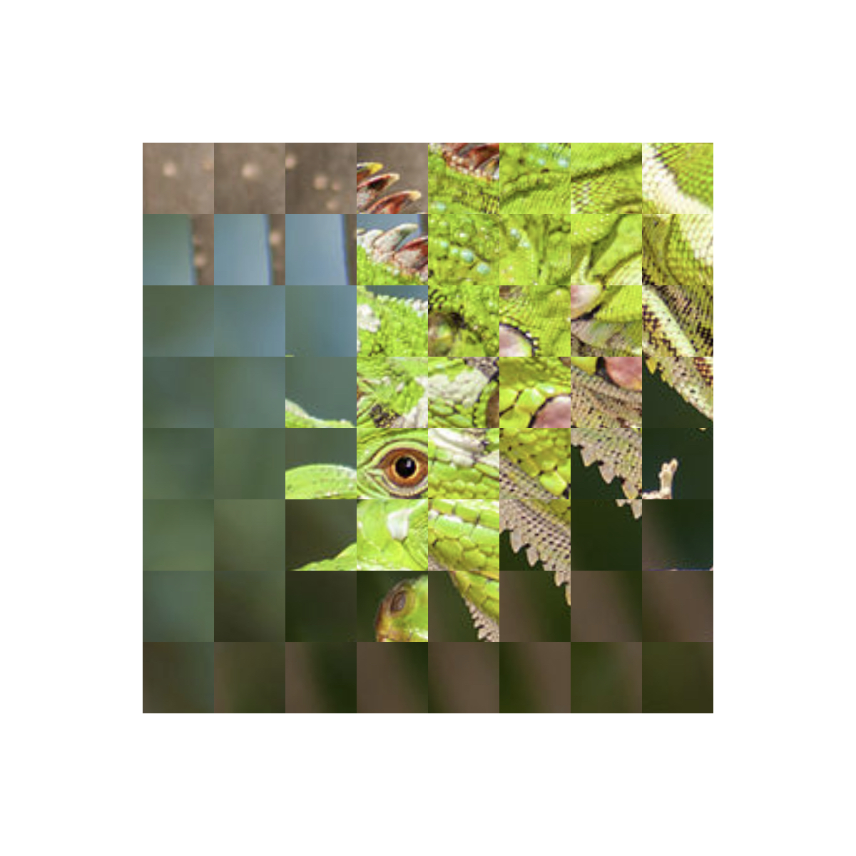
Then we can repeat this process by dissecting each of the four quadrants into quadrants themselves and rearranging these quadrants in the same way, and then dissecting and rearranging those quadrants, and so on. If we repeat this transformation one more time on the quadrants of this image, we get the following "second-generation" picture:

Something very interesting and unexpected happens when we repeat this process many times, but before giving it away, let's take a look at the code. Here's the first key function used in my code:

def draw_square_img(ctx, pos, side, img, corner):
    ctx.save()
    x0, y0 = pos
    xc, yc = corner
    ctx.move_to(x0, y0)
    ctx.line_to(x0 + side, y0)
    ctx.line_to(x0 + side, y0 + side)
    ctx.line_to(x0, y0 + side)
    ctx.line_to(x0, y0)
    picture = cairo.ImageSurface.create_from_png(img)
    ctx.set_source_surface(picture, xc, yc)
    ctx.clip()
    ctx.paint()
    ctx.restore()
    picture = 0

This function is pretty simple: given a coordinate position for the corner of the square pos = (x0, y0), a side length side, an image img, and another coordinate position corner = (xc, yc) for the corner of the image, this function paints a square section of that image. Cairo aligns a copy of the image such that its corner coincides with the point specified by pos, and then it will draw a square with side length side and a corner at the point corner and restrict the image to that square. This way, we can choose not only the position of the square, but also which piece of image appears in it.

The next function is where the interesting recursion happens:

def shuffled_img(ctx, depth, pos, side, img, corner):
    x0, y0 = pos
    xc, yc = corner
    if depth == 0:
        draw_square_img(ctx, pos, side, img, corner)
    else:
        shuffled_img(ctx, depth - 1, (x0, y0), side/2, img, (xc - side/2, yc - side/2))
        shuffled_img(ctx, depth - 1, (x0, y0 + side/2), side/2, img, (xc - side/2, yc + side/2))
        shuffled_img(ctx, depth - 1, (x0 + side/2, y0), side/2, img, (xc + side/2, yc - side/2))
        shuffled_img(ctx, depth - 1, (x0 + side/2, y0 + side/2), side/2, img, (xc +  side/2, yc + side/2))

The arguments of this function are the context ctx (as usual), the depth depth of the recursion, or the number of times the "shuffling" operation is to take place, the position pos of the corner of the square containing the final image, the side length side of the square containing the final image, the image img to be shuffled, and the position corner of the image's corner before it is restricted to the specified square. If depth is equal to zero, then no transformations are applied to the image, and so the function simply draws the image unaltered inside of a square with the specified parameters. However, if depth is greater than zero, four separate instances of this same function are called again, one for each of the squares four quadrants, each with the depth parameter decremented by one. This is where the recursion occurs - the function calls four separate instances of itself, each of which calls four separate instances of the function again, and so on, until depth reaches zero and each of the "subquadrants" is filled with an unaltered version of a section of the image.

All that we have to do now is create and call the main function.

 

def main():
    surface = cairo.ImageSurface(cairo.FORMAT_ARGB32, 1200, 1200)
    ctx = cairo.Context(surface)
    ctx.set_source_rgb(1, 1, 1)
    ctx.paint()
    shuffled_img(ctx, NUM_ITER, (200, 200), 800, "seeds/iguana.png", (0, 0))
    surface.write_to_png("gallery/shuffled_ig_"+str(NUM_ITER)+".png")
if name == "main":
    main()

As before, this function sets up the ImageSurface, creates a Cairo context, creates the background color, and generally sets everything up before calling the principal function. Then shuffled_img is called and saved to a PNG file. The variable NUM_ITER is a variable specifying the "depth" of image transformation, assigned elsewhere in the code.

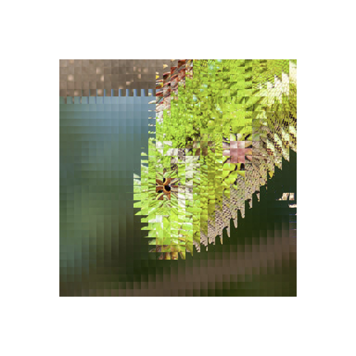
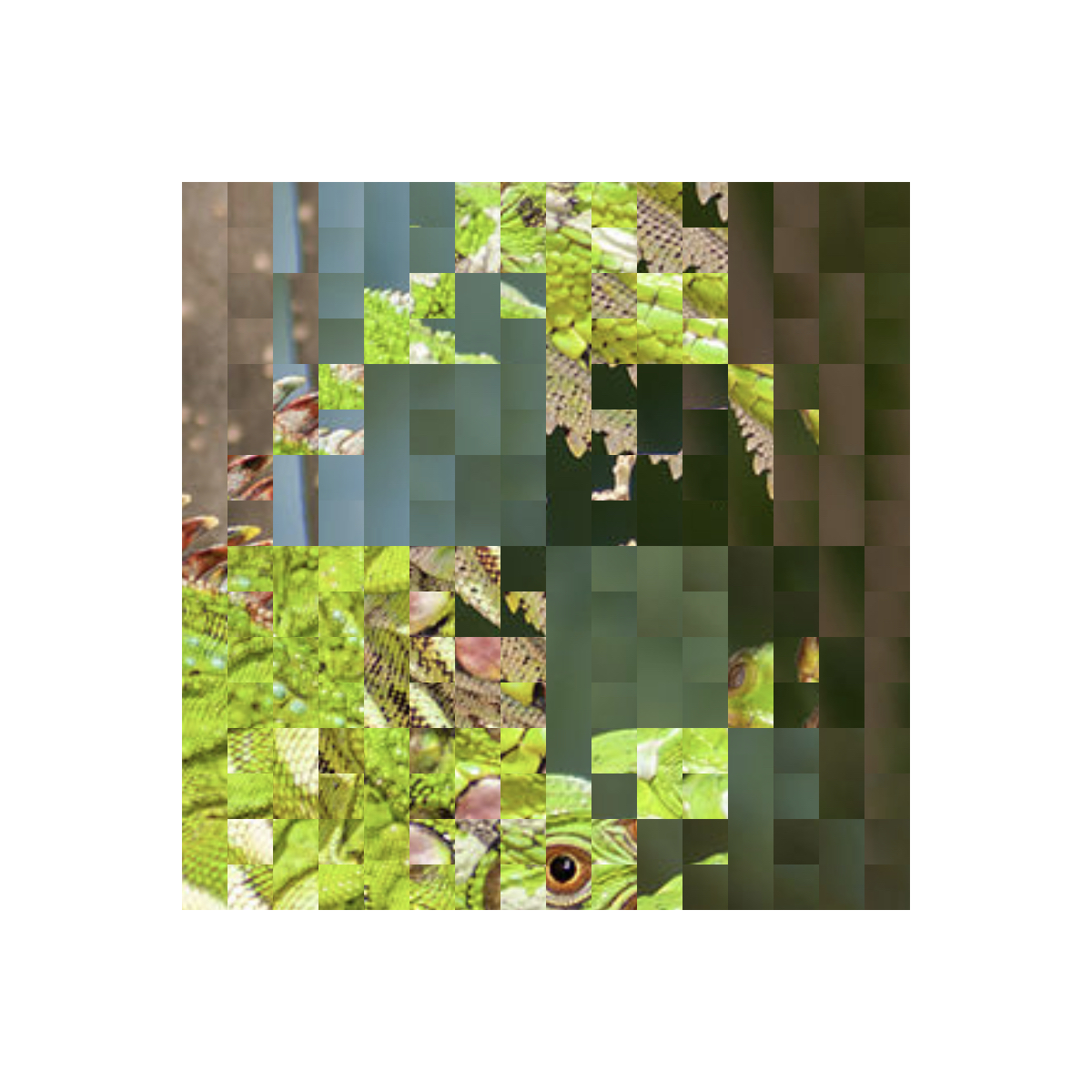
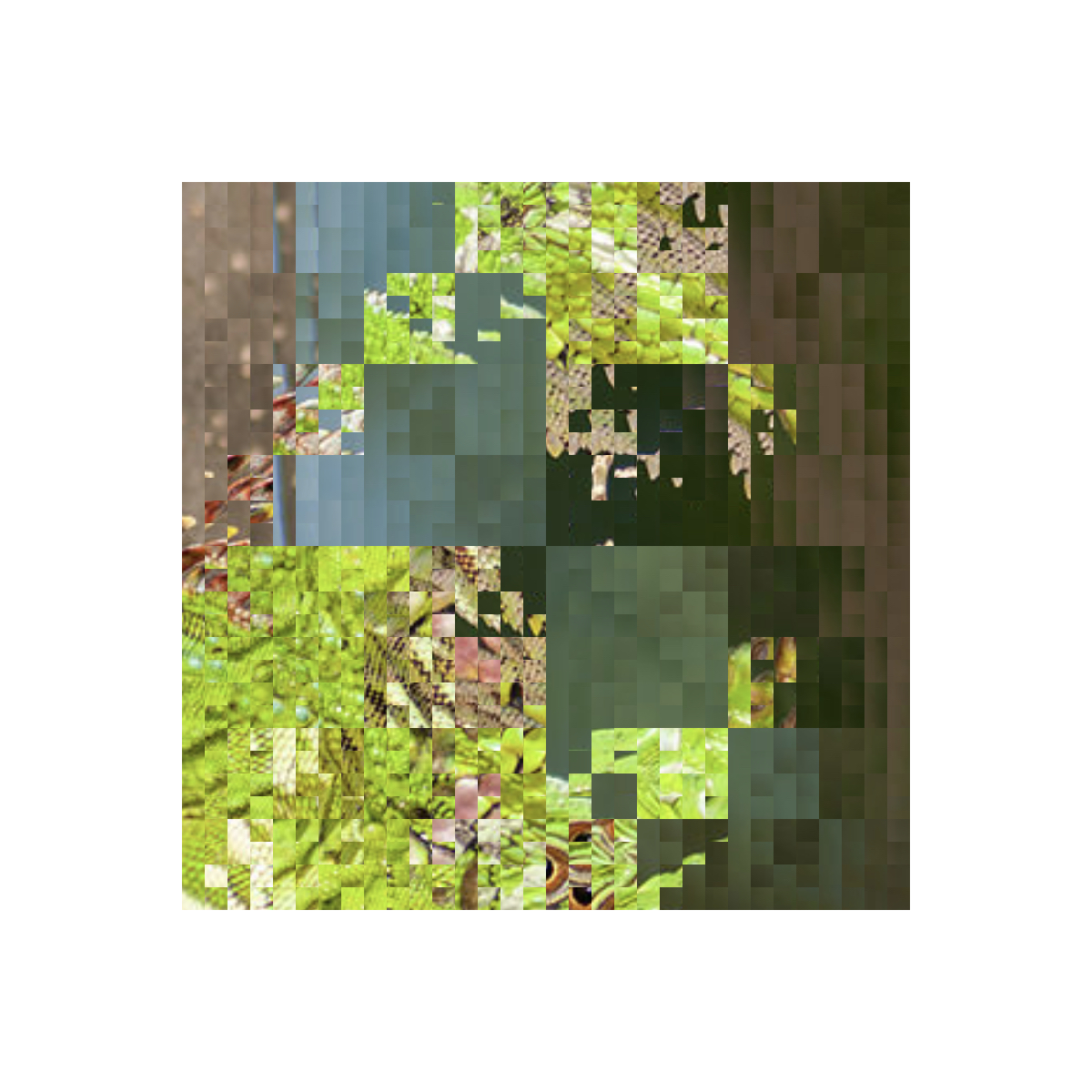
We're done! We've seen what the first- and second-generation images look like, so now let's see generations 3 through 6:

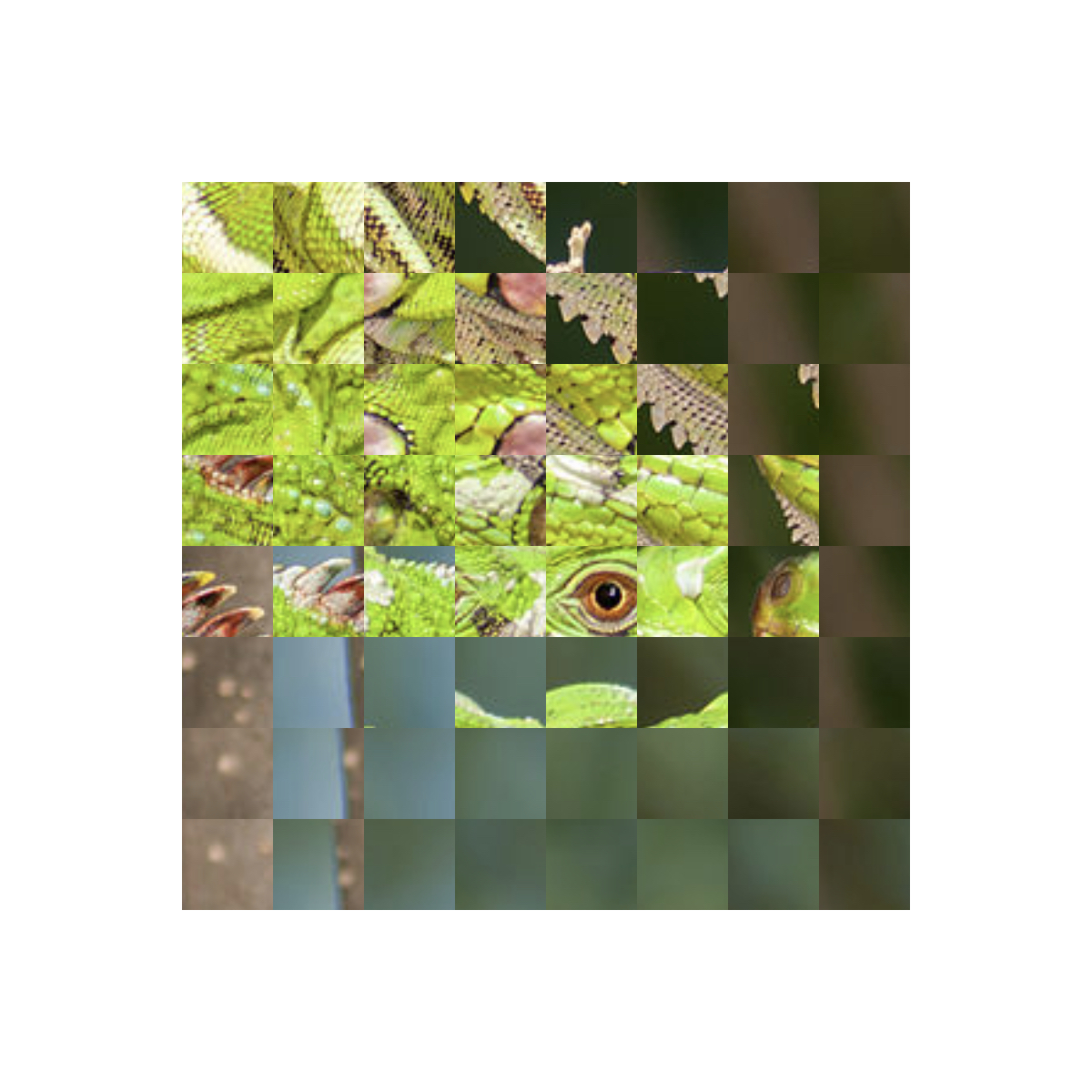
Do you see something strange happening here? The more times this transformation is applied, the more it looks like an inverted version of the original image! Can you figure out why this happens?

By making slight changes to the shuffled_img function, we can iterate different transformations as well. For example, consider the following alternate way of shuffling the four quadrants of a square:

Below are generations 2 though 6 of iterated shuffling:

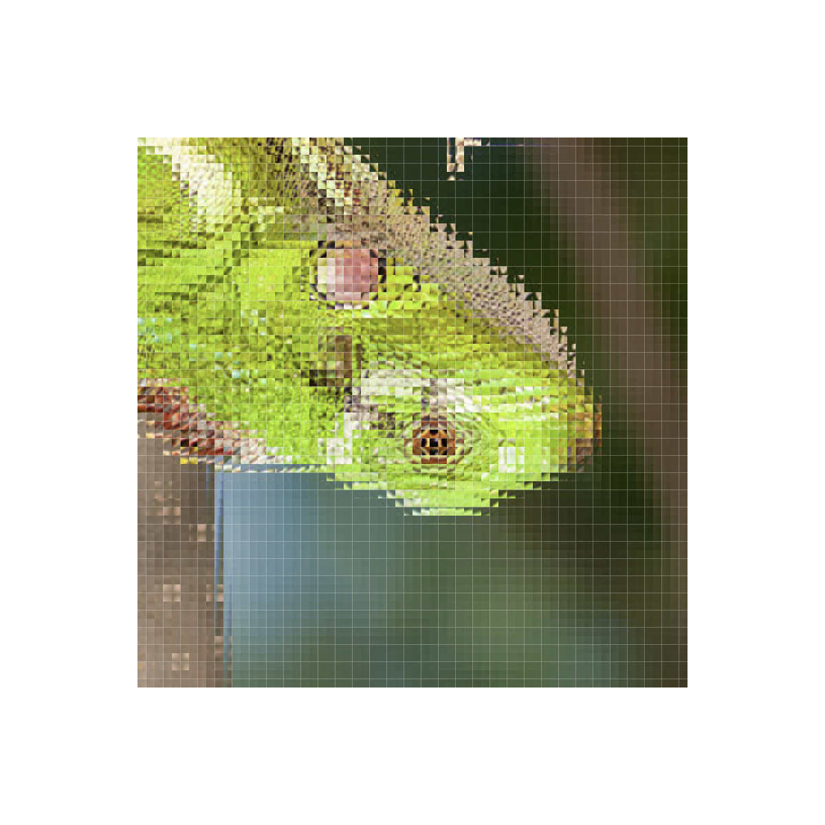
Once again, something recognizable has somehow emerged from apparent chaos - the longer we repeat the process, the more it appears that the image is just being rotated $90^\circ$ counterclockwise. Can you explain how the chosen permutation of quadrants caused this regular pattern to emerge?

Alright, so if recursively applying the previous two types of "shuffle" have respectively resulted in the image being inverted and rotated $90^\circ$ counterclockwise, can you predict what the image will look like after repeating the following "shuffle," without skipping ahead to look at the results?

If you think you've come up with a prediction, scroll down to see generations 2 through 6 of this type of shuffle:

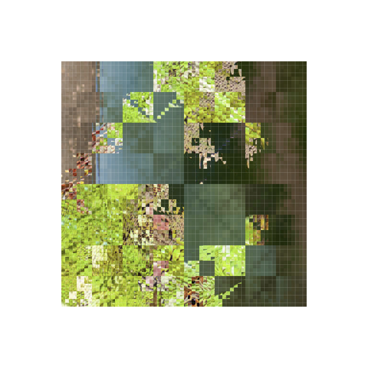
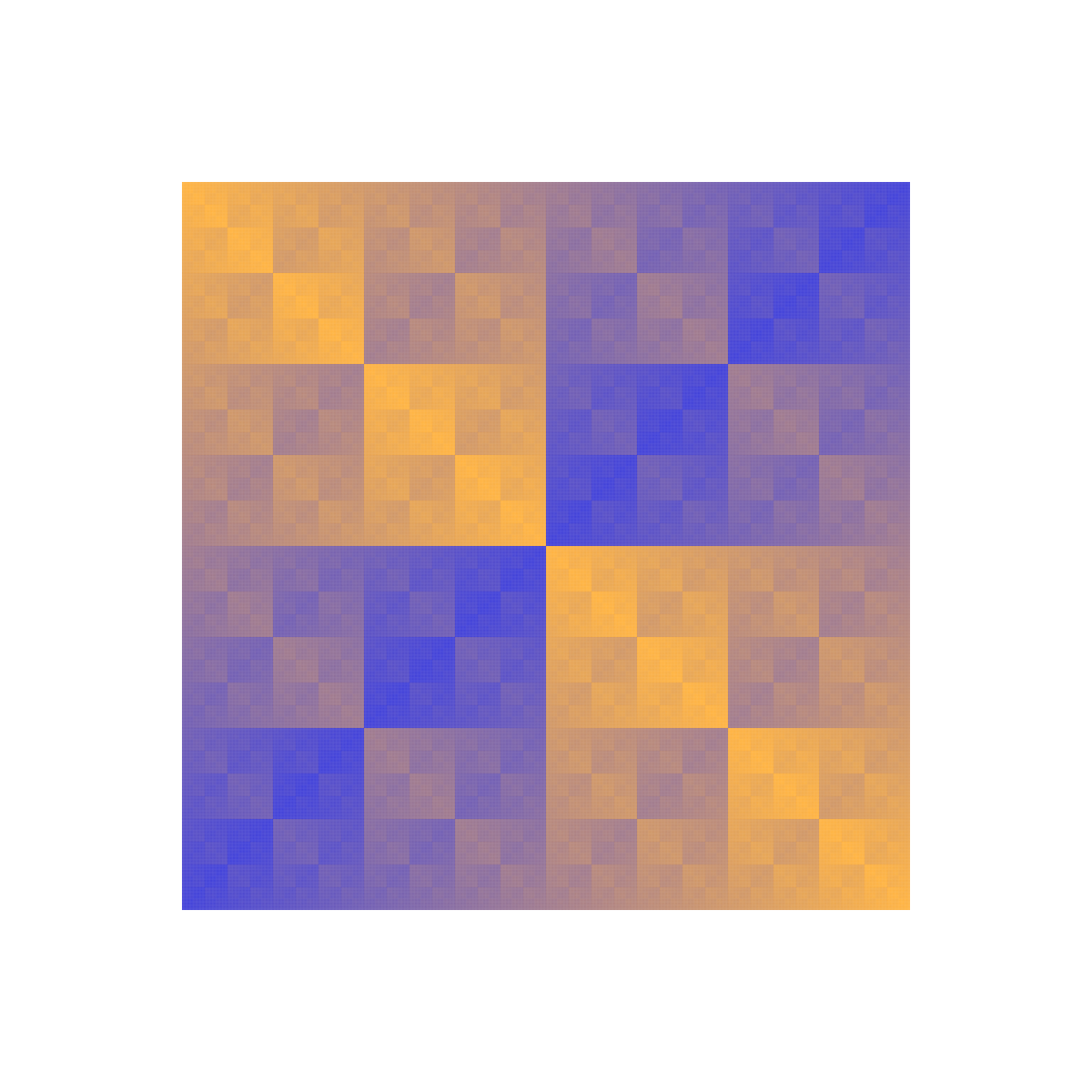
Okay, it was a trick question - this type of shuffle doesn't actually end up producing anything nice and regular, just a fractally scrambled mess. This doesn't suit our friend the iguana very well, but if we instead apply this transformation to a simple linear gradient between two colors, we end up with a beautiful and rather mesmerizing fractal of color:

Randomly Nested Boxes

The third and final class of generative geometrical art that we'll play with incorporates randomness in addition to recursivity. For that reason, it suggests all sorts of interesting probabilistic questions, so get ready for math puzzles.

Mondrian style art that consists of geometric shapes (specifically boxes) filled with solid colors lends itself to automatic generation with Pycairo. Although we're not going to try to imitate Mondrian, what we create here will be similar in that it will consist solely of monochromatic geometric shapes. It's easy to generate lots of random colored shapes, but the challenge is to make a program that generates pictures that are actually aesthetically pleasing.

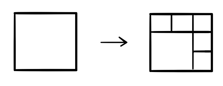
In this design, we'll start with an empty square, which is transformed in one of three different ways: either

• it is left completely empty, or
• it is divided into four square quadrants, or
• a colored circle is inscribed in the square.

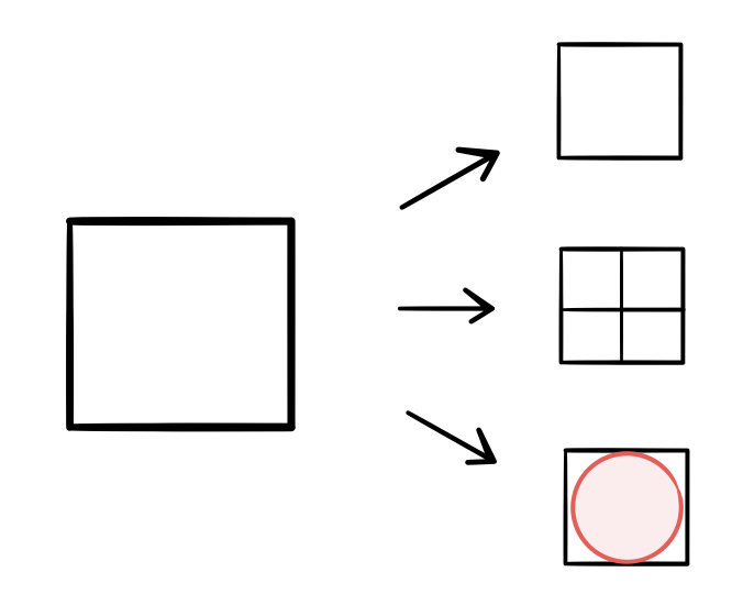
These transformations take place with respective probabilities $p_1$, $p_2$, and $p_3$ (such that $p_1 + p_2 + p3 = 1$). If the first or third transformations occur, the process terminates and the picture is finished. If the second transformation occurs, then the same process is applied to each of the four quadrants into which the square is divided. Clearly, this second transformation is where the recursion would take place in the code: the function that randomly applies one of these three transformations would have to call four more instances of itself (one for each quadrant) should the second transformation be randomly selected.

Because the code used to create these images is so similar to that used in the previous section, I won't go through it here (if you want, you can try creating it yourself as an exercise). However, there is one issue that should be addressed: how do we know that this process will terminate? Couldn't these squares go on splitting into quadrants forever, causing an infinite loop? In practice, this can be avoided by setting a minimum size for splitting (such that if a square's size is smaller than the minimum, it cannot divide into four quadrants). In theory, however, this gives rise to an interesting math problem.

If there were no minimum splitting size and the squares were free to split at arbitrarily small sizes, with a splitting probability of $p_2$, what would be the chance of an infinite loop? In other words, how likely would it be that the image produced by this process would have infinite depth? See if you can work out the answer yourself - I'll write out my solution after showing off some of the pictures produced by this process.

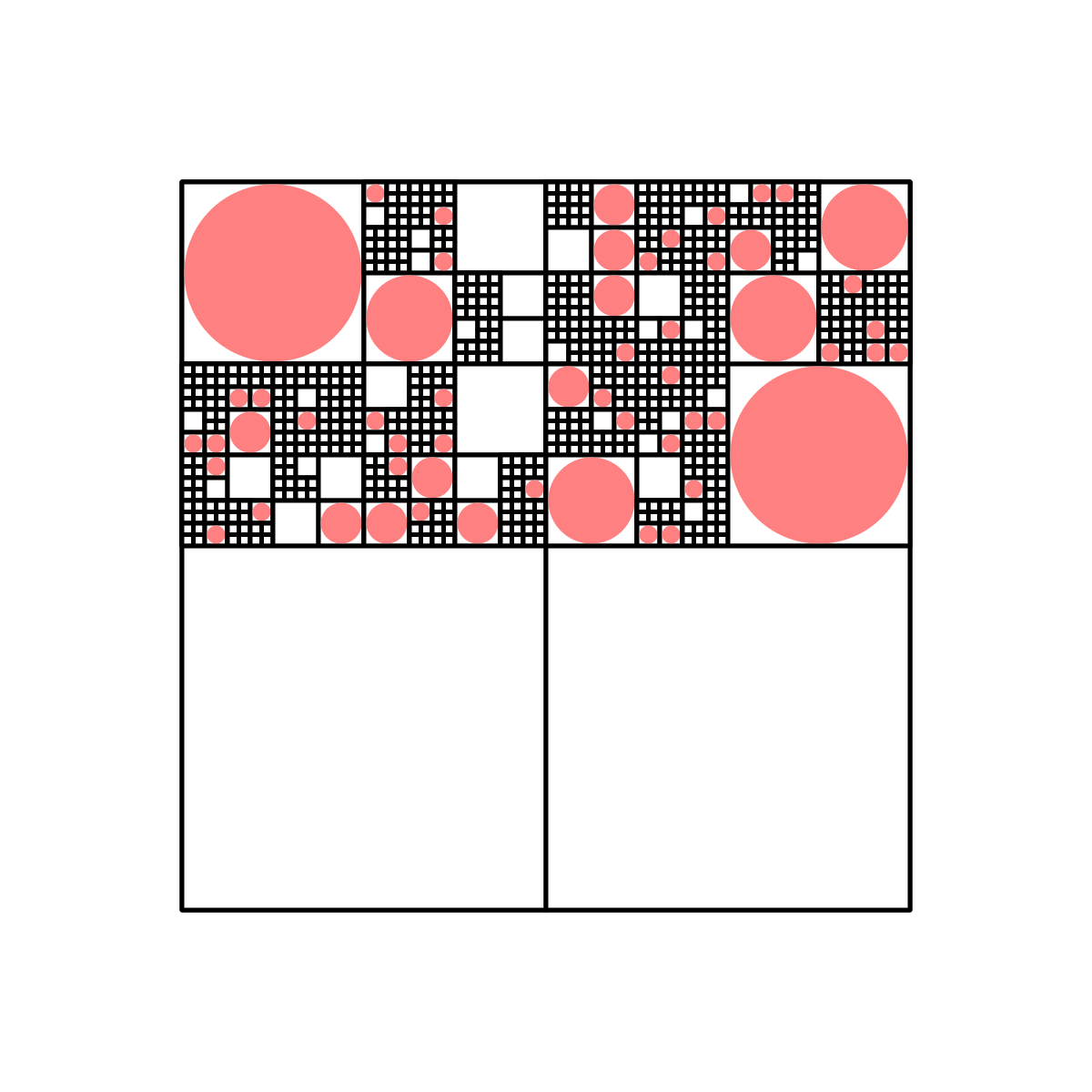
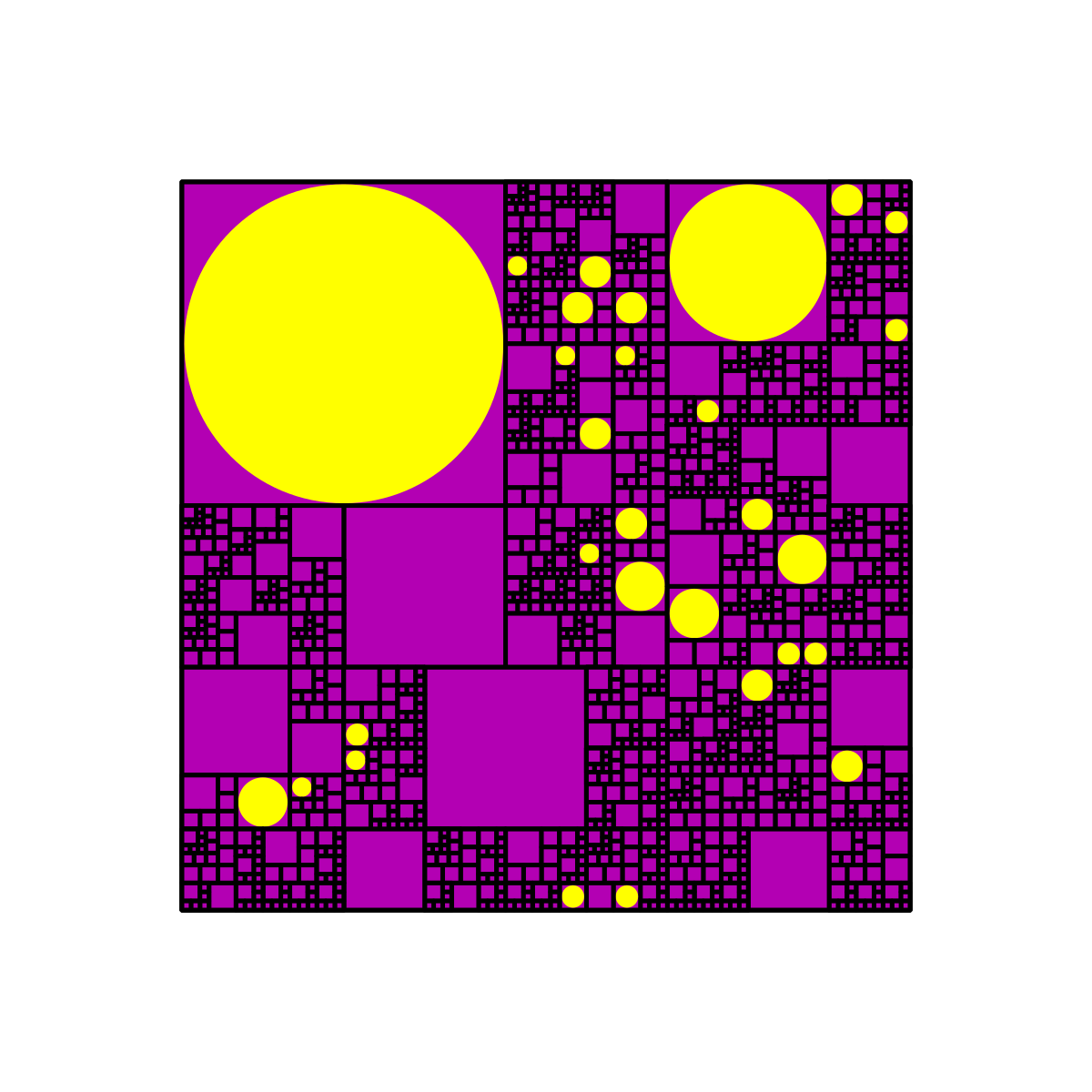
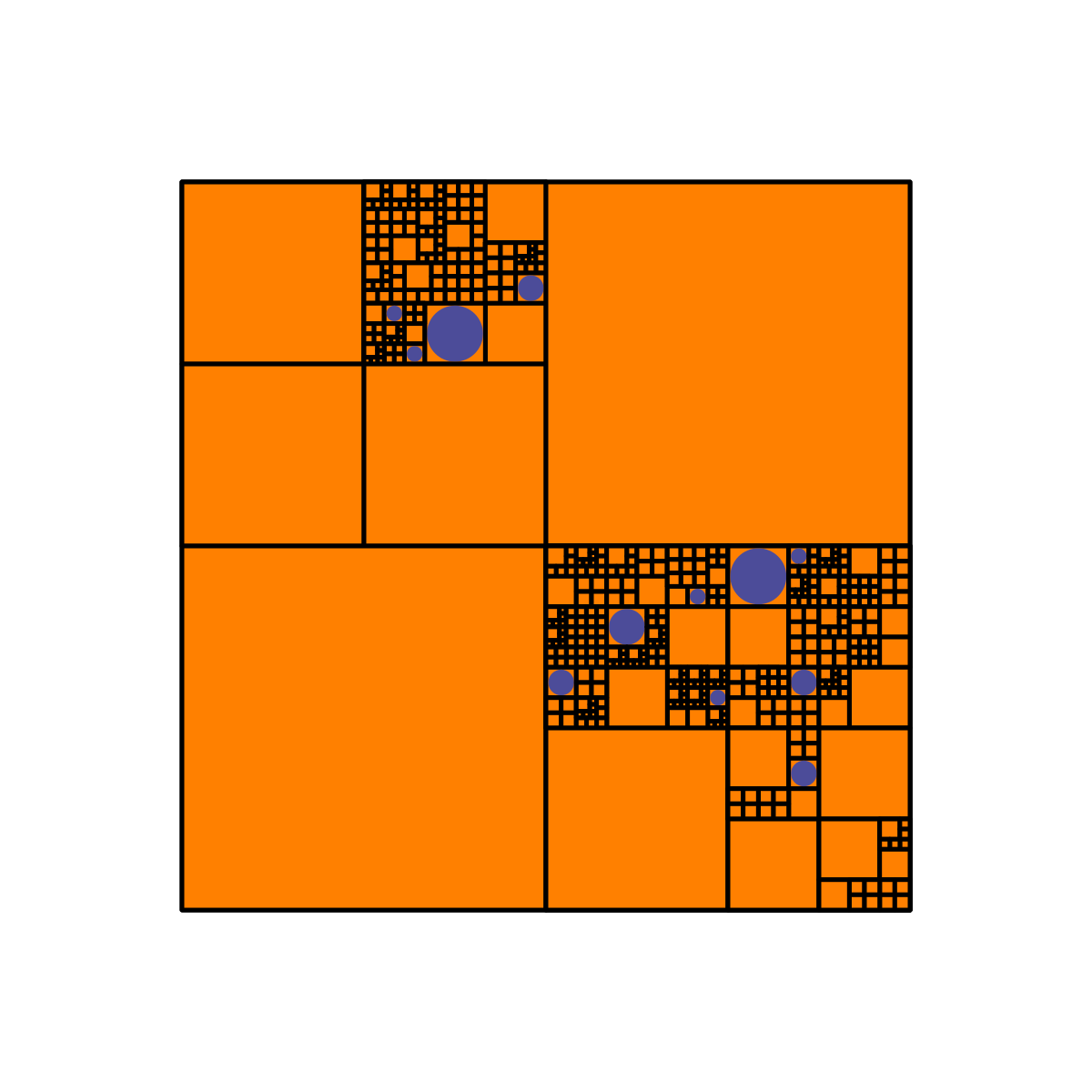
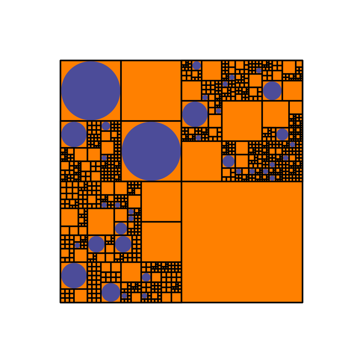
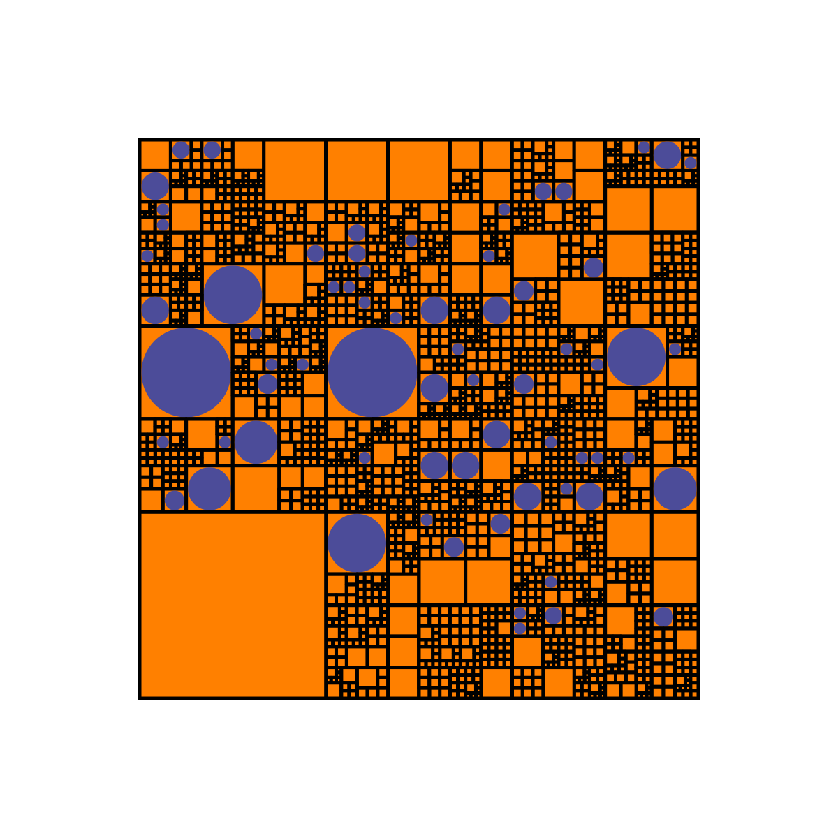
Here are some designs created with $(p_1, p_2, p_3) = (0.1, 0.7, 0.2)$:

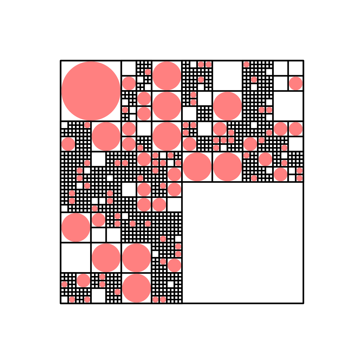
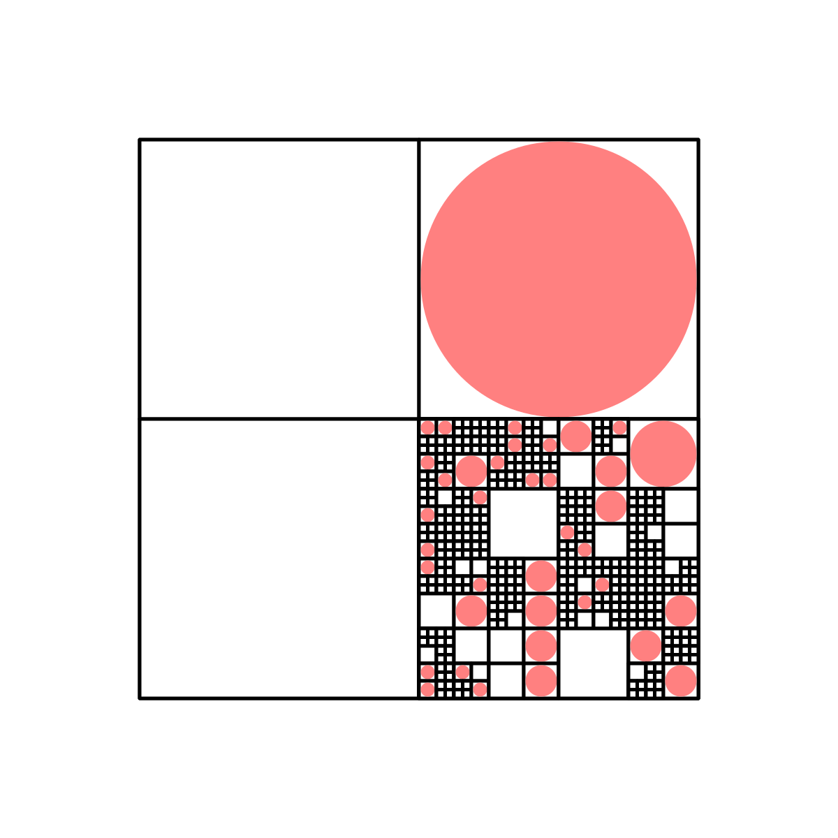
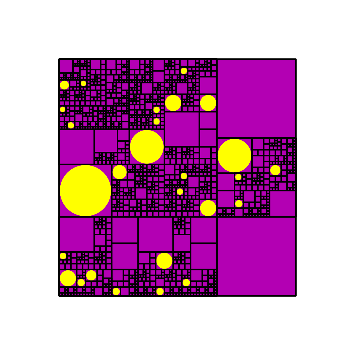
And here are some with $(p_1, p_2, p_3) = (0.3, 0.6, 0.1)$:

As you can see from the second example, there's always a chance that this program will output something "boring." This could be remedied by, say, forcing the original square to split at least a certain number of times, but we won't do that here, since we can always rerun the code if it produces insatisfactory results.

This can also be made more interesting by introducing new possible transformations. For example, in addition to the three we've been using so far, we could add this alternate splitting operation:

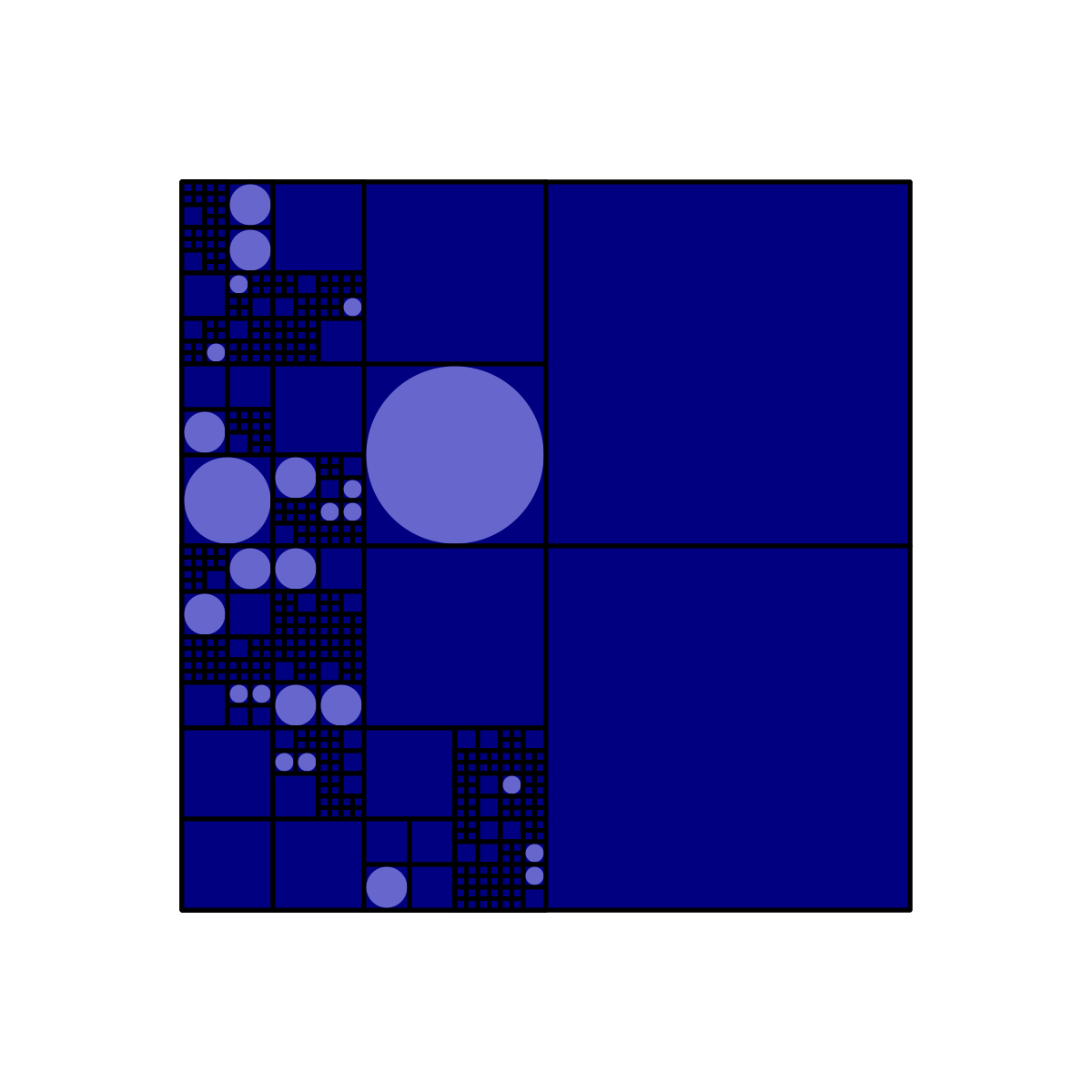
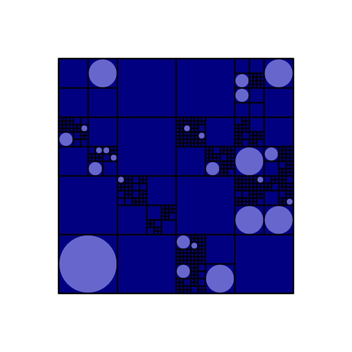
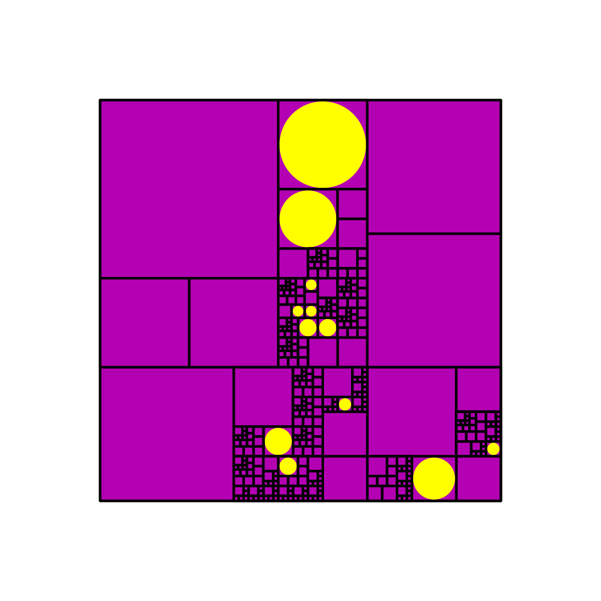
If we do this, we must introduce a fourth probability $p_4$ for this transformation, and impose the condition that $p_1+p_2+p_3+p_4=1$. For comparison with the earlier images that only used the four-quadrant split, here are three images formed using $(p_1, p_2, p_3, p_4) = (0.2, 0, 0.1, 0.7)$:

And here are three with $(p_1, p_2, p_3, p_4) = (0.2, 0.4, 0.1, 0.3)$:

I'm not sure why I find these designs so aesthetically pleasing and fun to look at - it probably has something to do with self-similarity and deeply nested levels of detail.

Okay, now time for some math! To restate the question from earlier: in the original version of the recursion (with only a four-quadrant split and no six-square split, i.e. $p_4=0$), given the value of $p_2$, what is the probability that the process repeats infinitely many times and the structure becomes infinitely "deep"?

Let $q$ be the probability of eventual termination. Obviously, the process terminates if it does not split on the very first iteration, and this occurs with probability $(1-p_2)$. Further, even if it splits (with probability $p_2$), it could still terminate if the subprocesses in each of the four quadrants terminates, which occurs with probability $q^4$. Therefore, we have that

$$q = 1-p_2 + p_2\cdot q^4$$

So the probability of eventual termination is the solution of the above quartic in $q$, which is bound to get a little bit messy (quartic equations are nasty to solve). However, we can neatly express $p_2$ in terms of $q$:

$$p_2 = \frac{1-q}{1-q^4} = \frac{1}{(1+q)(1+q^2)}$$

By plugging in possible values of $q$ like $q=1/2$ and calculating $p_2$ using the above equation, we can determine, for example, that setting $p_2 = 8/15$ results in a 50/50 chance of the process terminating. Furthermore, it tells us that if $p_2$ is less than $1/4$, then the process will terminate with probability $1$.

To conclude this blog post, here are two more probability puzzles about the process we've described in this section:

• In the original version described (with $p_4 = 0$), if $p_2 < 1/4$ and the process is guaranteed to terminate (with probability $1$), what is the expected number of circles, in terms of $p_2$ and $p_3$?
• In the original version of the process, let $c_0$ be the probability that the final image has $0$ circles and $c_1$ the probability that it has exactly $1$ circle. Calculate $c_1$ in terms of $p_2$, $p_3$, and $c_0$.